Fuzzy Logic
Fuzzy Logic is a representation of a model in linguistic variable and handling the fuzziness/vagueness of their value to take decisions. It removes the sharp boundaries to describe a stratification and allows overlapping. The main idea behind Fuzzy systems is that truth values (in fuzzy logic) or membership values are indicated by a value in the range [0, 1] with 0 for absolute falsity and 1 for absolute truth.
Fuzzy set theory differs from conventional set theory as it allows each element of a given set to belong to that set to some degree (0 to 1), unlike in conventional method the element either belongs to or not. For example if we calculated someone’s skill index as 3.9 and we have medium group which contains skill 2.5 to 4 and High group which contains 3.5 to 5. In this case the member is part of, Medium group has around 0.07 degree and High group around 0.22 (not calculated value). This shows the Fuzziness. Remember this is not probability but its certainty which shows degree of membership in a group.
In Fuzzy logic the problem is given in terms of linguistic variable, however the underlying solution is made of mathematical (numerical) relationship determined by Fuzzy rules (user given). For example, if Skill level is high and KEDB usage is High, then Turn-Around-Time (TAT) is Met is rule, for setting up this rule, we should study to what extent this has happened in the past. At the same time this will also be a part in Not met group of TAT to a degree.
In software we use Fuzziness of data (overlapping values) and not exactly the Fuzzy rules but we allow mathematical/stochastic relationship to determine the Y in most cases. We can say a partial application of Fuzzy logic with Monte Carlo simulation.
Fuzzy Logic- Sample
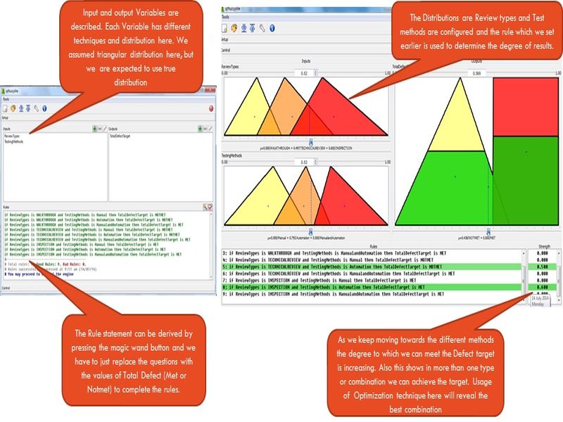
To understand the Fuzzy logic, we will use the tool qtfuzzylite in this case. Assume that a project is using different review techniques and able to find defects which are overlapping with each other’s output. Similarly they use different test methods and they also yield results which are overlapping with each other. The total defects found is the target and it’s met under a particular combination of review and Test method and we can use Fuzzy logic in modified form to demonstrate it.
Study the distributions by Review Type and configure them in input. If there is fuzziness among the data then there can be overlap
Study the Test method and their results, and configure their distribution in the tool
In output Window configures the Defect Target (Met/Not met) with target values.
The tool will help to form the rules with different combination and the user has to replace the question and give the expected target outcome.
In the control by moving the values of Review and Test method (especially in overlapping area) the tool generates certain score ,which tells about what will the degree of membership with met and Not met. The higher value combination out of these shows there is more association with results.
One of the way by which we can deploy this is by simulating this entire scenario multiple times and thereby making this as stochastic relationship than deterministic. This means use of Monte Carlo simulation to get the range of possible results or probability of meeting the target using Fuzzy logic.
Many a times we don’t apply Fuzzy logic to complete extent or model as it is in software industry, however the fuzziness of elements are taken and modelled using statistical or mathematical relationship to identify range of outputs . This is more of hybrid version than the true fuzzy logic modelling.
Fuzzy Logic – Sample
Monte Carlo Simulation
Monte Carlo simulation is used mainly to study the uncertainties in the value of interest. Its statistical method of simulation, which uses the distributions and randomness to perform simulation. In simulation model the assumptions of the system are built and a conceptual model is created, and using Monte Carlo method the system is studied using number of trials and variations in the distributions, which results into range of outputs.
For an example to study the life of a car engine, we can’t wait till it really gets wear out, but by using different conditions and assumptions the engine is simulated to undergo various conditions and the wear out time is noted. In Monte Carlo method, it’s like we test another 100 such engines and finally get the results plotted in histogram. The benefit is that this is not a single point of outcome, but it’s a range, so we can understand the variation with which the life of engine could vary. Similarly since we test many, we can understand the probability of an engine having a life beyond a particular value (ex: 15 years).
The computers have made the life easy for us, so instead of struggling for 100 outcomes, we can simulate 5000, 10000 or any number of trials using the Monte Carlo tools. This method has helped us to convert the mathematical and deterministic relationship to be made as stochastic model by allowing range /distributions of factors involved them, there by getting the outcome also under a range.
The model gives us the probability of achieving a target, which is in other words the uncertainty level.
Assume a deterministic relationship of Design Effort (X1) + Code Effort (X2) = Overall Effort(Y), which can be made as stochastic relationship by building the assumptions (variation of X1 & X2 and distribution) of variables X1, X2 and running the simulation for 1000 times and storing all the results of Y and building histogram from it. Now what we will get is a range of Y. The input variation of X1 and X2 is selected randomly from the given range of X1 and X2. For example if code effort varies from (10, 45) hrs then any random values will be selected to feed into equation and get a value of Y.
Monte Carlo technique can be demonstrated using Excel formulas also, however we will discuss the relevant topics based on crystal ball (from Oracle) tool, which is another excel plug in.
Performing simulation:
The data of any variable can be studied for its distribution and central tendency and variation using Minitab or excel formula.
The influencing variable names are entered (X’s) in excel cells and their assumptions (where distributions and their values) are given
Define the outcome variable(Y) and in the next cell give the relationship of X’s with Y. It can be a regression formula or mathematical equation etc (with mapping of X’s assumption cell in to the formula)
Define the outcome variable formula cell as Forecast Cell. It would require just naming the cell and providing a unit of outcome.
In the preferences, we can set any number of simulations we want the tool to perform. If there are many X’s, then increase simulation from 1000 to 10000 etc. Keep a thumb rule of 1000 simulation per X.
Start the simulation, the tool will run the simulations one by one and keeps the outcome in memory and then plots a Histogram of probability of occurrence with values. We can give our LSL / USL targets manually and understand the certainty by % or vice versa. This helps us to understand the Risk against achieving the target.
Optimization:
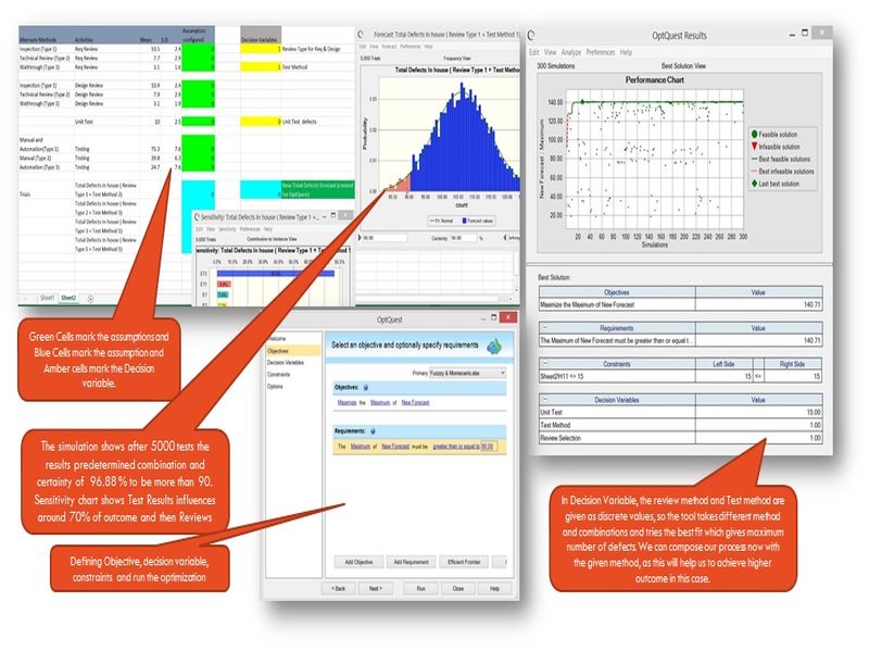
Though in simulation we might have seen the uncertainty of outcome, we have to remember that some X’s are controllable (Hopefully we have modelled that way) and by controlling them, we can achieve better outcome. OptQuest feature in the tool helps us to achieve the optimization by picking the right combination of X’s.
At-least one Decision Variable has to be created to run OptQuest. Decision variables are nothing but controllable variables, and without them we can’t optimize.
Define the Objective (maximize/minimize/etc with or without a LSL/USL) and tool detects Decision Variables automatically. We can introduce constraints in decision variables (Ex: A particular range within with it has to simulate). Run Simulation (Optimization is based on simulation), the tool runs with random picking values within the range of decision variables and records the outcome and for best combination of X’s for which target of Y is met, it keeps that as best choice, until something more better comes within the cycles of simulation.
The best combinations of X’s are nothing but our target values to be achieved in project and the processes which have capability to achieve these X’s are composed in Project.
Monte Carlo Simulation- SAMPLE
A Project team receives and works on medium size (200-250 FP) development activities and whenever their internal defects exceeds more than 90 or to a higher value, they have seen that UAT results in less defects. They use different techniques of review and testing based on nature of work/sub domains and each method gives overlapping results of defect identified and there is no distinctness in their range. Now we are expected to find their certainty of finding defects more than 90 and to see what combination of review and test type, the project will find more defects.
Tools like JMP, Processmodel, BaysiaLab has in built simulation features within them and there we don’t need to use Crystal ball kind of tool.
Recently in Minitab 17, we have profilers and optimizers added in the regression models, which reduce the need of additional tools. However it has limitation of only for Regression.
Simulacion is a free tool and it has an acceptable usage with up-to 65000 iterations and 150 input variable. This is another Excel Add on.
Risk Analyzer is another tool which is similar in Crystal ball and is capable of performing most of the actions. However this is paid software.
There are many free excel plugins are available to do Monte Carlo simulation and we can also build our own simulation macros using excel.
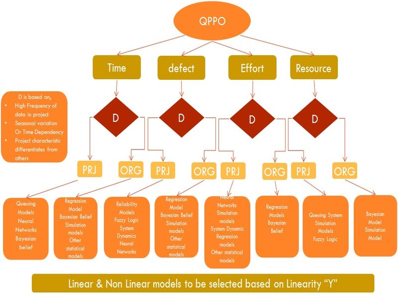
PRO-Project and ORG –Organizational Level
Key Characteristics to determine model
Robustness of model
Prediction Accuracy of model
Flexibility in varying the factors in model
Calibration abilities of the model
Availability of relevant tool for building the model
Availability of data in the prescribed manner
Data type of the variable and factors involved in the model
Ability to include all critical factors in the primary data type (not to convert in to a different scale)
PPM for Selected Cases:
So the cases where Defect Density and SLA Compliance are the QPPOs and their relevant Process/Sub Processes are selected with measures to monitor (Logically), its time to find the relationship and make them as suitable Process Performance Models. The Model should be able to comply the practices given in last few sections.
Defect Density (Y) and X Factors
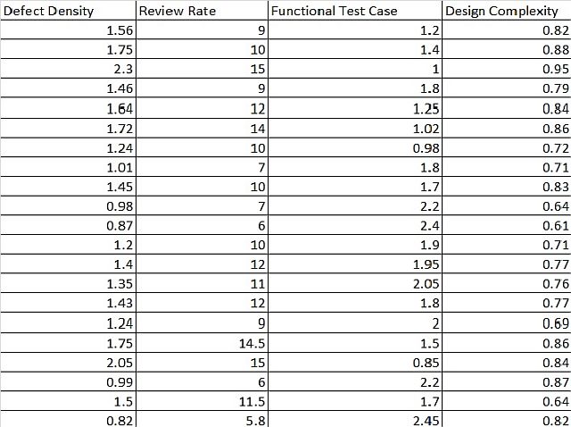
With the above given data from different Project Release outcomes, we will use regression technique to build the Process Performance Model.
Regression Analysis: Defect Density versus Review Rate, Functional Test , Design Complexit
Analysis of Variance
Source DF Adj SS Adj MS F-Value P-Value
Regression 3 2.56507 0.85502 45.70 0.000
Review Rate 1 0.42894 0.42894 22.93 0.000
Functional Test Case 1 0.09107 0.09107 4.87 0.041
Design Complexity 1 0.11550 0.11550 6.17 0.024
Error 17 0.31805 0.01871
Total 20 2.88312
Model Summary
S R-sq R-sq(adj) R-sq(pred)
0.136780 88.97% 87.02% 80.34%
Coefficients
Term Coef SE Coef T-Value P-Value VIF
Constant 0.227 0.442 0.51 0.614
Review Rate 0.0750 0.0157 4.79 0.000 2.24
Functional Test Case -0.2143 0.0971 -2.21 0.041 2.35
Design Complexity 0.994 0.400 2.48 0.024 1.39
Regression Equation
Defect Density = 0.227 + 0.0750 Review Rate - 0.2143 Functional Test Case
+ 0.994 Design Complexity
Fits and Diagnostics for Unusual Observations
Defect
Obs Density Fit Resid Std Resid
7 1.2400 1.4831 -0.2431 -2.27 R
R Large residual
We have got a fit regression equation with one data point showing large residual.
For SLA Compliance QPPO, we have collected monthly compliance of few projects,
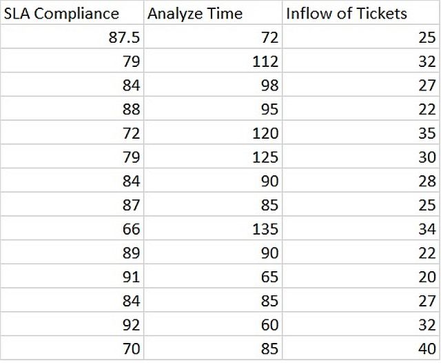
Using Regression Technique
Regression Analysis: SLA Compliance versus Analyze Time, Inflow of Tickets
Analysis of Variance
Source DF Adj SS Adj MS F-Value P-Value
Regression 2 730.4 365.19 33.64 0.000
Analyze Time 1 188.3 188.26 17.34 0.002
Inflow of Tickets 1 246.2 246.24 22.68 0.001
Error 11 119.4 10.86
Total 13 849.8
Model Summary
S R-sq R-sq(adj) R-sq(pred)
3.29487 85.95% 83.39% 64.33%
Coefficients
Term Coef SE Coef T-Value P-Value VIF
Constant 123.92 5.17 23.98 0.000
Analyze Time -0.1875 0.0450 -4.16 0.002 1.20
Inflow of Tickets -0.841 0.177 -4.76 0.001 1.20
Regression Equation
SLA Compliance = 123.92 - 0.1875 Analyze Time - 0.841 Inflow of Tickets
Fits and Diagnostics for Unusual Observations
SLA Std
Obs Compliance Fit Resid Resid
13 92.00 85.77 6.23 2.43 R
R Large residual
We have got a fit regression equation with one residual point. These equations can be used as process performance model, as long as similar conditions and within the boundary value of X factors, another project performs.
What We Covered:
Organizational Process Performance
SP1.5 Establish Process Performance Models