![]()
5 Electrostatic application: calculating and analyzing fields
In this chapter, we will use the mesh file we created to find a field solution. To get started, run EStat from the TriComp program launcher. Click the 1 tool and choose the Mesh file CoaxialCylinders.MOU. The program determines the defined regions in the mesh and displays the dialog of Fig. 20. The values shown are appropriate to the solution parameters discussed in the previous chapter. Fill in the fields and click OK, accepting the output file name CoaxialCylinders.EIN (EStat Input).
To understand the action of the dialog, choose File/Edit script (EIN) and load the file in the editor. Here is the content:
* File: CoaxialCylinders.EIN Mesh = CoaxialCylinders Geometry = Rect
DUnit = 1.0000E+02
ResTarget = 5.0000E-08
MaxCycle = 5000
* Region 1: DIELECTRIC Epsi(1) = 1.0000E+00
* Region 2: INNERELECTRODE Potential(2) = 1.0000E+02
* Region 3: OUTERBOUNDARY Potential(3) = 0.0000E+00
EndFile
You’ll recognize many of the entries. The ResTarget and MaxCycle parameters that control the solution accuracy are described in the EStat manual. The default values are fine for this calculation.
Exit the editor and click the 2 tool. After you choose CoaxialCylinders.EIN, EStat generates and solves the finite-element equations in less than a second. Larger meshes will take longer, but generally the run times of practical solutions are less than a minute. The program creates the files CoaxialCylinders.ELS (a diagnostic listing file that you can inspect with an editor) and CoaxialCylinders.EOU (a record of the mesh coordinates and potential values at the nodes).
To see the results, press the 3 tool and choose CoaxialCylinders.EOU. You can generate interesting plots in the Analysis menu (Fig. 21). For this discussion, let’s concentrate on hard numbers. First, let’s check the absolute accuracy of the solution with a single point calculation. At radius r = 10.0 cm, the formulas listed in the previous article give the values:
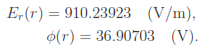
Numerical interpolations in EStat involve the collection of potential values from surround- ing nodes. On symmetry boundaries, there are only half the available nodes, so the accuracy is not optimal. We should use an internal point for a good comparison. On a 45o line, the
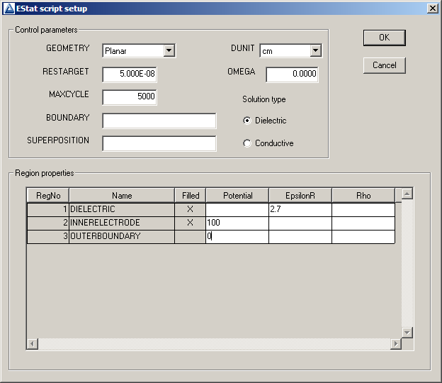
Figure 20: Dialog to create the EStat input script.
position r = 10.0 cm corresponds to x = y = 7.071068 cm. Click the Point calculation tool. We can specify the location by moving the mouse inside the solution volume and clicking the left button. This selection method is not accurate enough for the comparison. Instead, press the F1 key after starting the Point calculation tool to enter coordinates manually. Fill in the x-y values and click OK. Values of several calculated quantities are displayed at the bottom. The calculated values of potential (36.90767 V) and electric field (910.23111 V/m) agree with the theoretical value to within thousands of a percent.
Rather than copy numbers from the screen, why not let EStat write them for us? Click the Open data record command and accept the default name CoaxialCylinders.DAT. Now, every time we do an interactive calculation, the results are recorded in the text file. For example, choose the menu command Analysis/Volume integrals. You can inspect the resulting file with an external editor. To use the internal EStat editor, click the Close data record command first (two instances of a same file cannot be opened simultanously in a program). Open the data file to see the result of the field-energy calculation (volume integrals of the field-energy-density):
Quantity: Energy
Global integral: 1.708936E-07
RegNo Integral
==========================
1 1.708936E-07
2 9.881184E-37
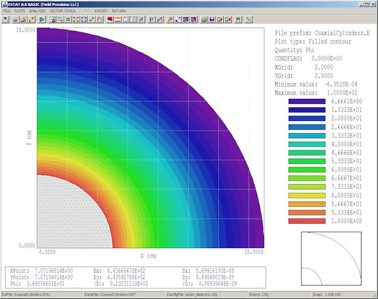
Figure 21: Filled-contour plot of potential with results of a point calculation displayed.
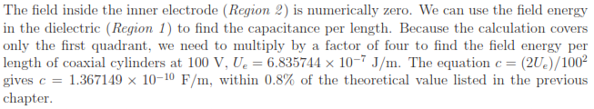
To understand the effects of element size, we want to compare accuracy at several radii for different choices of element dimensions. The procedure would be tedious if we had to run the Point calculation tool and type coordinates for each datum. In the next chapter, we’ll automate the analysis procedure.