![]()
6 Electrostatic application: meshing and accuracy
In this chapter we’ll continue with the solution of the previous chapter, making several calcu- lations to understand the effect of element size on solution accuracy. To expand our toolbox of techniques, we’ll automate steps in the analysis procedure. The best way to start a project is with a clear statement of the goal. In this case, we want to check the accuracy of numerical estimates of the electric field Er(r) at locations in the dielectric as a function of element size. Specifically, we’ll check field interpolations near the inner electrode (r = 5.0 cm), near the outer electrode (r = 15.0 cm) and at the center of the gap (r = 10.0 cm) for the following choices of approximate element size: 0.1 cm, 0.2 cm, 0.3 cm, 0.4 cm and 0.5 cm.
As mentioned in previous chapters, good supporting software (text editors, file managers, image editors,...) is essential for effective technical work. In this case, we’ll use a spreadsheet created with OpenOffice Calc. Figure 22 shows the upper section of the sheet. Parameters at the top include the inner and outer radii, the applied voltage and the theoretical value for the capacitance per length in z. The section beneath lists the radial positions for the calculations. Note that the inner radius is slightly larger than ri and the outer radius smaller than ro. Remember that the electrode boundaries are a set of straight lines that approximate sections of circles. We have to include a little slack to make sure that the test points lie within the dielectric region for all choices of element size. We may as well let the spreadsheet do the mathematical work. The cells for the x-y coordinates of the measurement points on a 45o line contain the formula r/√2. Similarly, the cells for the theoretical values contain the equations for Er(r) and φ(r) discussed in the previous chapters.
The section below the theoretical values illustrates another use of spreadsheets. Why not let the program prepare the input scripts? In this case, we’ll generate an analysis script – a set of instructions to EStat for standard calculations to carry out for each of the solutions:
* Coaxial cylinders analysis script
INPUT COAXIALCYLINDERS.EOU OUTPUT COAXIALCYLINDERS.DAT POINT 3.53624 3.53624
POINT 7.07107 7.07107
POINT 10.60589 10.60589
VOLUMEINT 1
ENDFILE
The spreadsheet has supplied the coordinates. To use the information, simply copy it and paste it into a text file CoaxialCylinders.SCR (SCRipt). The commands have the following actions:
• Open the EStat output file CoaxialCylinders.EOU.
• Write the results of calculations to CoaxialCylinders.DAT.
• Perform three point interpolations at the desired locations.
• Calculate volume-integral quantities over Region 1 to find the capacitance per length.
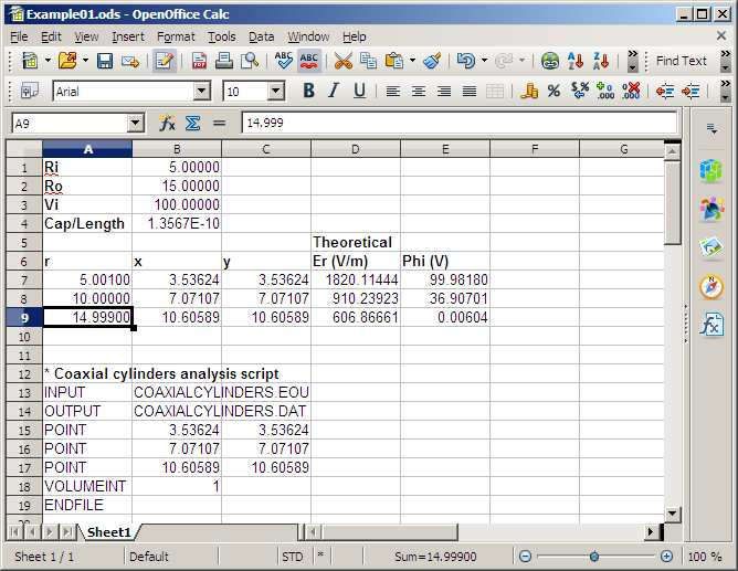
Figure 22: Top section of a Calc spreadsheet: solution setup
We can quickly change the element size by editing the Mesh input script. Figure 23 shows the file displayed in the Context editor. The red arrows show the quantities to be modified. Given a modified Mesh input script, there are three steps to regenerate the solution and set new values in the data file CoaxialCylinders.DAT:
• Run Mesh, load CoaxialCylinders.MIN, process the mesh and save the result.
• Run EStat, load CoaxialCylinders.EIN and run the solution.
• Run the analysis script CoaxialCylinders.SCR.
With only five solutions, the procedure wouldn’t take long. On the other hand, it takes only a few seconds to set up a Windows batch file that handles everything automatically.
In the Tricomp Program Launcher (tc.exe), press the Create task button to bring up the dialog of Fig. 24. Fill in the file prefix CoaxialCylinders and activate the Beep at completion box. We need to define the three tasks of a solution. Clicking a cell in the first column raises a popup menu (inset) that shows your installed Field Precision programs as well as useful batch commands. For the first task, choose Mesh. Then, click in the second column and choose the Select file button. The program displays a standard dialog to select appropriate input files with suffix MIN. Pick CoaxialCylinders.MIN to fill in the first row. Similarly, define two more tasks for an EStat solution and an analysis. When the display looks like Fig. 24, press OK. The program creates the file CoaxialCylinders.BAT in the working directory. Here is the content:
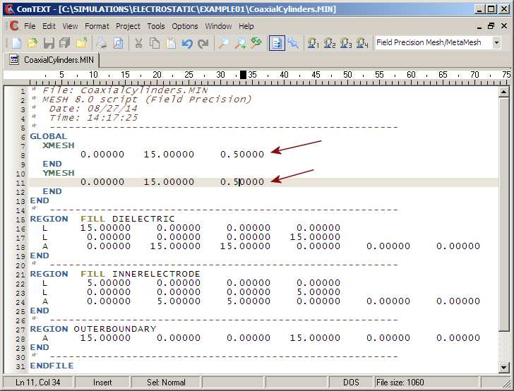
Figure 23: File CoaxialCylinders.MIN displayed in Context.
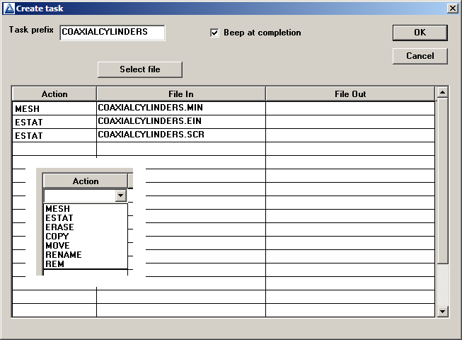
Figure 24: Create task dialog in tc.exe.
REM TriComp batch file, Field Precision
START /B /WAIT C:fieldp_basictricompmesh.exe COAXIALCYLINDERS
START /B /WAIT C:fieldp_basictricompestat.exe COAXIALCYLINDERS.EIN
START /B /WAIT C:fieldp_basictricompestat.exe COAXIALCYLINDERS.SCR
START /B /WAIT C:fieldp_basictricompNOTIFY.EXE
IF EXIST COAXIALCYLINDERS.ACTIVE ERASE COAXIALCYLINDERS.ACTIVE
Note that most Field Precision programs can run from the command line with the input file as a heading parameter. The /WAIT option ensures that a program does not start before the previous program completes it action. Under batch file control, a full solution consists of the following users operations:
• Edit and save CoaxialCylinders.MIN with the desired element size.
• Press Run task in the program launcher and choose CoaxialCylinders.BAT.
• Edit the resulting file CoaxialCylinders.DAT and extract values of interest.
I performed the solutions and copied and pasted values to create the sections of the spread- sheet shown in Fig. 25. I also set up formulas in the spreadsheet to determine the relative errors in electric-field values. For a visual reference, Fig. 26 shows the mesh for element sizes of 0.2 and 0.5 cm. We can now consider some implications of the results:
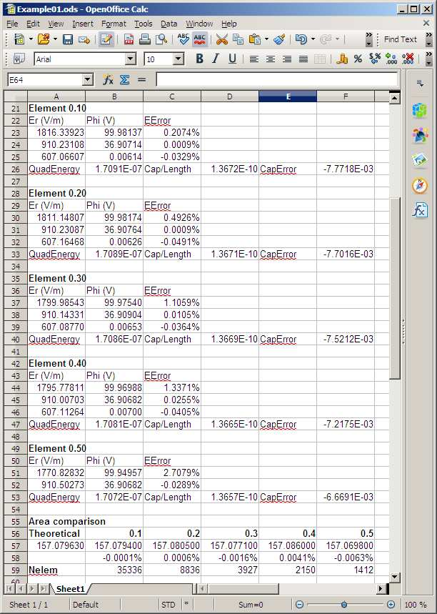
Figure 25: Bottom section of a Calc spreadsheet: solution analysis.
• For an element size of 0.1 cm, the mesh had 35336 elements. The mesh with size 0.5 cm had only 1412 elements. Therefore, the solution with the fine mesh required about 25 times as much computational work.
• The error in the electric field calculation at the center of the gap (r = 10.0 cm) was infinitesimal for element size 0.1 cm (0.0009%) and acceptable for many applications at 0.5 cm (0.0289%).
• The error in electrical field near the electrodes was higher, as we would expect when representing a curved surface with a set of line segments. The relative error was higher on the inner electrode because there were fewer segments. For the 0.5 cm elements, the error of 2.7% on the inner electrode could be of concern for some applications.
Beginning users often employ far more elements than is necessary. For the determination of electric field values in the dielectric volume (removed from electrodes), the accuracy with the fine mesh of Fig. 26 may not justify the extra computational work. If you have concerns about mesh resolution, the standard procedure is to do two calculations with different mesh sizes and to check whether values in critical regions differ by more than the accuracy requirement. Note that there are two techniques to increase accuracy while minimizing the number of element:
• Use variable mesh resolution.
• Use the Boundary method to create a microscopic solution within a macroscopic solution.
Variable resolution is discussed in Chap. 8. The boundary method, an advanced technique to resolve small features in a large solution space, is covered in the instruction manuals for EStat, PerMag, HiPhi and Magnum.
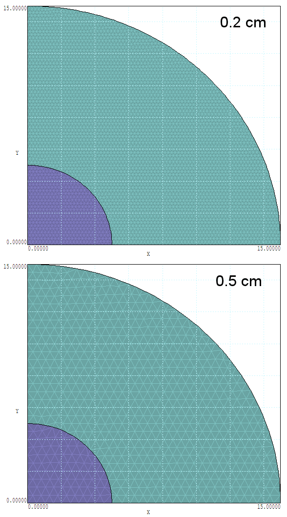
Figure 26: Mesh geometries for small and large elements.
We’ve covered a lot of ground in the last three chapters following a simple electrostatic solution:
• Organizing simulation data and using a file manager.
• Defining region boundaries with the Mesh Drawing Editor.
• Employing symmetry boundaries to reduce the size of a calculation.
• Using a spreadsheet to plan and to analyze calculations.
• Understanding the set of input and output files for an electrostatic solution.
• Creating program input scripts in interactive dialogs and modifying them with a text editor.
• Generating and inspecting standard mesh definition files with Mesh.
• Defining run-control and material parameters for EStat solutions.
• Running Mesh and EStat interactively or from the Windows command prompt.
• Automatically controlling EStat with analysis scripts.
• Creating batch files for automatic run control with the task generator of the TriComp
program launcher.
• Gaining insights into the relationship between element size and interpolation accuracy. In the next chapter, we’ll turn our attention to 2D magnet-field calculations.