![]()
4 Electrostatic application: building the mesh
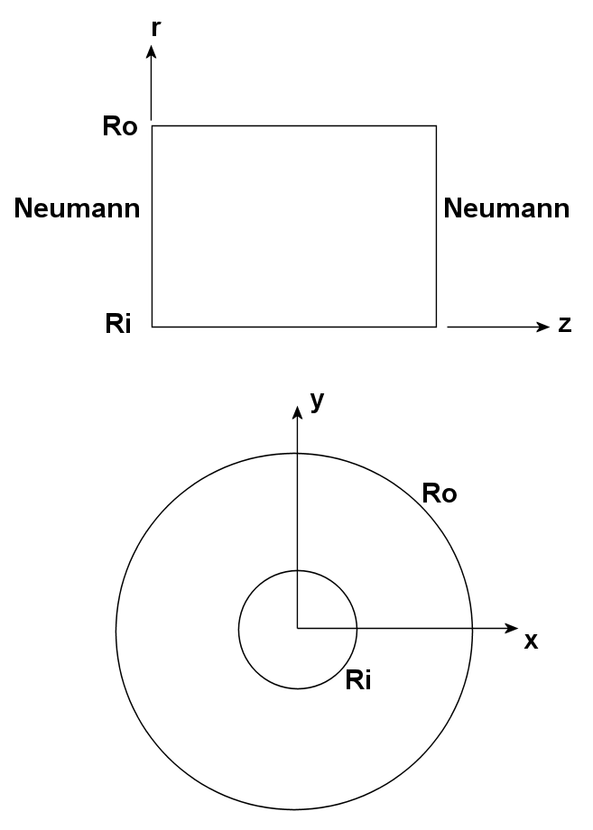
Figure 14: Alternative ways to model coaxial cylinders with a 2D code.
In the previous chapter, we followed a prepared example without going into the details of how the input files were prepared and how the mesh parameters were chosen. Now, we’re ready to build a complete calculation and learn about how the geometry of the mesh affects the accuracy of the solution. The best approach to make comparisons is to model a system that has an analytic solution. A good choice is a set of coaxial cylindrers with an applied voltage which have spatial variations of potential and electric field.
There are two ways to model coaxial cylinders with a 2D code (Fig. 14). The first is to use cylindrical coordinates z-r and to model the infinite length in z with Neumann conditions1 at the upper and lower z boundaries. This approach, where the electrode boundaries are simply straight lines, would not exercise the conformal mesh capability. Instead, we will use planar coordinates (Fig. 14, lower) where the cross section is in the x-y plane and the system extends infinitely in z (out of the page). For specific parameters, take ri = 5.0 cm, ro = 15.0 cm and Vi = 100.0 V. The space between the cylinders is filled with polyethylene (ǫr = 2.7) and the outer electrode is grounded. Using formulas available in introductory electromagnetism texts,
1The Neumann condition specifies that the parallel component of electric field, Ez, is zero at the boundaries.
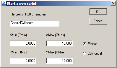
Figure 15: Dialog to start an interactive drawing session.
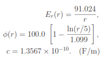
the radial variation of potential and electric field and the capacitance per unit length is given by:
To start, we will define the geometry for the numerical calculation. Run the Mesh program and choose File/Create script/Create script graphics. Fill out the dialog entries as shown in Fig. 15. For the dimensions given, note that the solution volume covers only the first quadrant of the space. We shall apply symmetry to reduce the amount of work – why calculate all four quadrants when the solution is the same in each one?
When you click OK, the program enters the drawing editor of Fig. 16. The display includes a menu at the top, a set of useful drawing tools beneath it, the main drawing area and a status bar at the bottom. We will define the following physical regions:
• Region 1: the polyethylene dielectric between the cylinders.
• Region 2: the inner boundary at 100.0 V.
• Region 3: the outer boundary at 0.0 V.
It is important to note that as we enter regions in sequence, the present region over-writes any shared elements or nodes of previous ones.
By default, the drawing editor is ready to add outline vectors for Region 1. Click the Line tool and move the mouse cursor into the drawing area. Note that the cursor changes to a cross and that there is an orange box showing the current coordinates. Snap mode is in effect by default, and the box moves in discrete steps to exact coordinate locations. Move the mouse cursor to the origin (x = 0.0, y = 0.0) and then click the left mouse button to set to start point of a line vector. Then move to the end of the x axis (x = 15.0, y = 0.0) and click the button again to set the end point. A line in the color of Region 1 appears along the bottom.
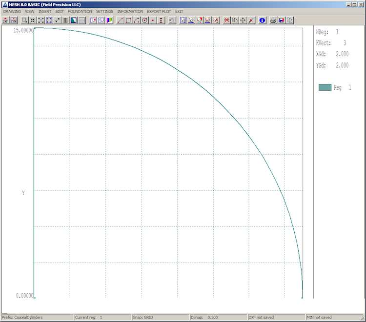
Figure 16: The Mesh drawing editor.
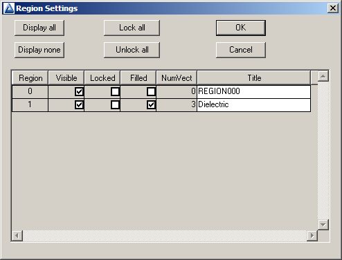
Figure 17: Region properties dialog.
The program remains in line entry mode. Draw another vector along the y axis from [0.0, 0.0] to [0.0, 15.0]. Right click the mouse to exit line entry mode. To add the circular edge of the region, choose the Arc/Start-end-center tool. Move the mouse to the following locations in sequence and click the left button at each one: [15.0, 0.0], [0.0, 15.0], [0.0, 0.0]. You should see the arc vector of Fig. 16.
With the outline of Region 1 complete, we shall set the region properties. Choose Set- tings/Region properties to bring up the dialog of Fig. 17. Region 0 is a special place to store reference vectors that will not appear in the output script. Supply the name Dielectric for Region 1 and check the Filled box. For a filled region, Mesh assigns not only the nodes of the boundary to Region 1, but also the elements enclosed. The Filled property applies to regions with non-zero volume. Exit the dialog.
Next, we are going to create the inner electrode by over-writing a portion of the dielectric volume. Click the Start next region tool, Now, all vectors you enter will be associated with Region 2. This region has the same shape as Region 1 except that the radius is 5.0 rather than 15.0. Use the same procedure except the first line should extend from [0.0, 0.0] to [5.0, 0.0] and so forth. When complete, go to Settings/Region properties. Assign the name InnerElectrode to Region 2 and set the Filled property. Exit the dialog.
To check the work so far, click the Toggle fill display tool to bring up the plot of Figure 18. The fill display mode is both a diagnostic and a visual aid. It checks that the vectors of filled regions define a closed surface and shows how the enclosed elements have been assigned. Click the tool again to return to the normal vector display.
We’ll conclude by defining Region 3. This region is not a filled volume but rather a set of nodes set to the fixed-potential condition on the outer boundary. We call such a region an un-filled or line region. Click the Start next region tool and then the Arc/Start-End-Center tool. Move to the following coordinates in sequence and click the left mouse button: [15.0, 0.0], [0.0, 15.0], [0.0, 0.0]. The nodes on the outer edge of Region 1 are re-assigned to Region 3 (color-coded violet). Set the region name to OuterBoundary and be sure that the Filled box in unchecked. You may ask whether it’s necessary to set special conditions on the dielectric
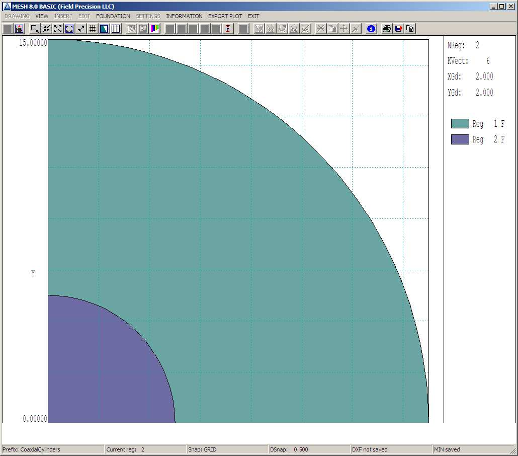
Figure 18: Checking the integrity of filled Regions 1 and 2.
boundaries on the bottom and left sides. A useful feature of finite-element solutions is that unspecified boundaries automatically assume the Neumann condition, exactly what we what. We’ll simply leave the boundaries alone.
Click the Export MIN tool to save a copy of the work and then exit the drawing editor. To see the result of the work, choose File/Edit file and pick CoaxialCylinders.MIN. Here is the content:
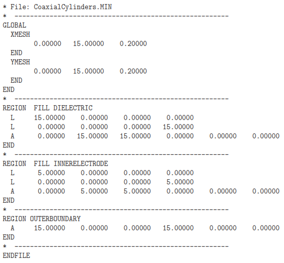
The region vectors and coordinates should look familiar. The commands at the top set the target element sizes. For now, we’ll accept the defaults.
The final step is generate a mesh file (CoaxialCylinders.MOU) from the region bound- ary specifications (CoaxialCylinders.MIN). In the main Mesh menu, choose File/Load/Load script (MIN) and pick the file you just created. Choose Process and then Plot-repair to view the result (Fig. 19). Is it a good mesh? Qualitatively, the answer is yes because the boundaries are relatively smooth and all features are well resolved (i.e., spatial variations of potential will be spread over many elements). We shall make this conclusion more quantitative in future articles.
In the next chapter, we will use the mesh for field calculations and comparisons.
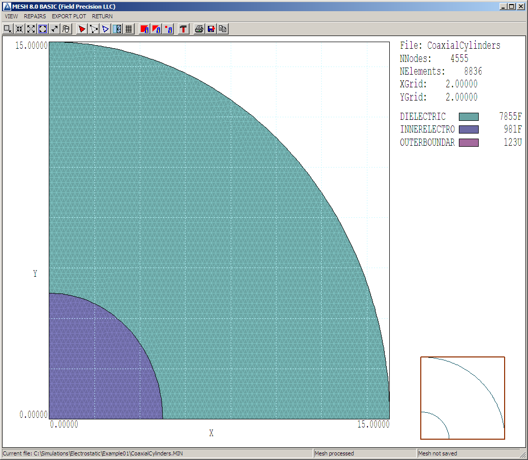
Figure 19: Completed mesh.