![]()
7 Magnetostatic solution: simple coil with boundaries
In this chapter, we’ll advance to 2D magnetostatic solutions using the programs Mesh and PerMag. The previous chapters on electrostatics have covered background on the basic con- cepts of finite-element calculations and the operation sequences of the programs. Therefore, in this chapter and following ones, we’ll concentrate on the special features of magnetic field calculations.
To review, finite-element solutions of the the previous chapters determined the electrostatic potential φ (a scalar quantity) at the node points of the mesh that we created. Components of the electric field vector at a location could then be determined by collecting local values of φ and taking numerical derivatives:
E = −∇φ. (3)
The components are Ex and Ey for planar solutions and Ez and Er for cylindrical solutions. Things get more involved for magnetic field calculations. The calculated node quantity is the vector potential A. The magnetic flux density B is given by
B = ∇ × A. (4)
Fortunately, there is only a single component of A in 2D calculations. The node quantity is Az for planar solutions (with flux density components Bx and By) and rAθ for cylindrical solutions (with components Bz and Br). The vector potential has useful properties for making plots:
• In planar solutions, contours of Az separated by a uniform interval ∆Az lie along lines of B separated by equal intervals of magnetic flux per length.
• In cylindrical solutions, contours of rAθ separated by a uniform intervals ∆(rAθ) lie along lines of B separated by equal intervals of magnetic flux.
Let’s get to work and generate some magnetic fields. We’ll start with a cylindrical coil in free space. Because the geometry is simple, we’ll write the boundary specifications directly. Run Mesh and click the New mesh (text) tool to bring up the dialog of Fig. 27. The values define a solution volume that covers the range -10.0 cm ≤ z ≤ 10.0 cm, 0.0 cm ≤ r ≤ 15.0 cm . When you click OK, the program opens the internal text editor with the default content shown in Fig. 28. The Global section at the top sets the foundation mesh (the set of elements before conformal shifting of boundary nodes). It covers the range we specified with a default element size of 0.1 cm. Advanced commands (like TriType) are listed as comment lines. We won’t need them for this calculation, so delete the comments.
A default region named SolVolume (Region 1 ) covers the solution volume, appropriate for this calculation3. Mesh has also started a default second region. We’ll use it to define the rectangular cross section of a cylindrical coil. The comment lines show the entries that could appear within a region section. Erase the comments and rename the region Coil. The coil has
2Mesh displays an error message if you try to open a cylindrical solution with r < 0.0.
3Although Region 1 often covers the full solution, it is not a necessary condition as we saw in the previous electrostatic solution.
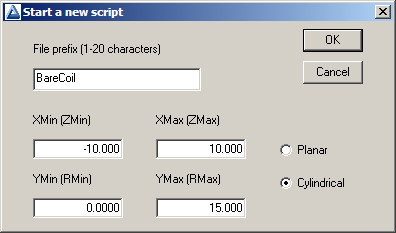
Figure 27: Dialog to start a Mesh script in the text mode.
dimensions -3.0 cm ≤ z ≤ 3.0 cm and 4.0 cm ≤ r ≤ 6.0 cm. Copy and paste the line vectors of Region 1 and use Search/Replace to modify the dimensions. We’ll also add a third region by copying and pasting Region 1 verbatim. Rename it Boundary and remove the word Fill in the Region command. We’ll discuss the purpose of this extra region later. For now, the modified script should look like Table 1. Save your work and exit the editor.
Click the Load script (MIN) tool to read the boundary specifications and then click Process. When complete, click Save mesh (MOU) to create the file BareCoil.MOU for use by PerMag. You can go to the Plot/Repair menu tool to view a cross-section of the resulting mesh, consisting of 60,000 elements.
Run PerMag and click the 1 tool to bring up the dialog of Fig. 29. As in the previous calculation, this dialog creates a script of run and material parameters to control the solution program. We can ignore several of the fields because the values control advanced runs with non-linear materials (e.g., saturable iron). For this run, we need only set the Geometry to Cylindrical and fill in the magnetic properties of the regions. Air has relative permeability µr = 1.0. The coil also has µr = 1.0. In addition, we need to set a total current that flows in the θ direction for a cylindrical solution. If the coil has N = 1000 turns and the drive current is I = 2.0 A, then the total A-turns over the cross section is 2000.0. Equivalently, the region carries a uniform azimuthal current density4 of 2000/[(0.06)(0.02)] = 1.667 MA/m2. Finally, we want to see what happens if we make no special provisions for the Boundary region, so don’t set any property. Click OK and save the data in the file BareCoil.PIN. You can check the file content with the internal PerMag editor.
Click the 2 button and choose BareCoil.PIN to create a finite-element solution. Then click 3 and load BareCoil.POU to analyze the solution. To begin, let’s check the lines of B. Click the Plot type tool and set the option Contour lines. Then click the Plot quantity tool and choose rAThet to produce the plot of Fig. 30a. There are two interesting features:
4Regions in PerMag always have uniform average current density. To represent a coil with variations of winding density, divide it into multiple regions.
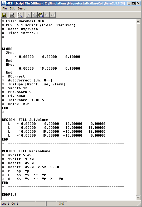
Figure 28: Starting a Mesh script in text mode, display of the internal editor.
Table 1: Mesh script BareCoil.MIN.
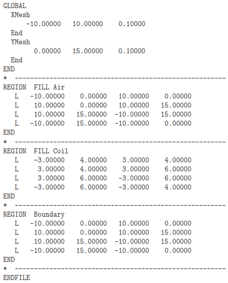
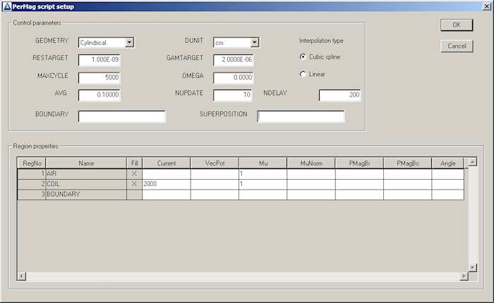
Figure 29: PerMag dialog to define run parameters and material properties.
• Even though the field inside the coil is fairly uniform, the space between lines is larger near the axis. This is because the lines are separated by intervals of equal magnetic flux and the area normal to z gets smaller as r approaches zero. In other words, the density of lines is not proportional to |B| in cylindrical coordinates.
• The lines of B are normal to the boundaries, the standard default Neumann condition for a finite-element magnetic solution (i.e., the derivative of vector potential normal to the boundary is zero). With regard to the axial boundaries, the condition would occur if there were an infinite array of coils with alternating positive and negative currently. Certainly, this is not what we intended. Furthermore, the boundary on the outer radius is non-physical in the sense that we could find no set of real coils that would generate the field pattern.
With regard to the second point, we must clearly do some thinking about the boundary condition. The alternative is to set the vector potential equal to a constant on the boundary. The Dirichlet condition is rAθ = 0.0. In this case, the component of B normal to boundary is zero, so that lines of B are parallel. To do this, we change the specification of Region 3 to:
The command states that the node quantity assumes a fixed value.
Figure 30b shows the modified solution. It is better in one respect. The field pattern could be achieved in an actual physical system: a coil inside a superconducting can. At this point, you may object that you wanted a coil in infinite space, not in an enclosure. This illustrates a limitation of the finite-element method. Calculations must be performed in a finite volume.
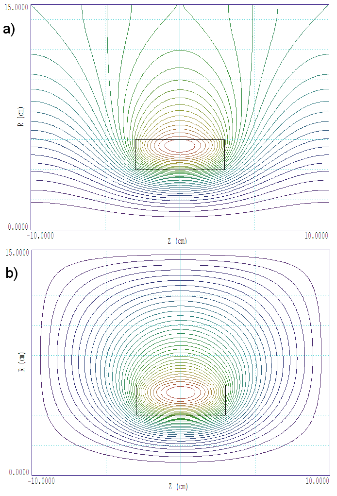
Figure 30: Lines of B for the solution. a) Default Neumann boundary condition. b) Dirichlet condition, fixed vector potential.
There will be boundaries, and conditions on the boundaries must be specified. The common conditions are Neumann or Dirichlet.
But, is it a limitation? Sometimes, issues in a numerical solution mirror issues in the physical world. When is the last time you operated a magnet in infinite space? In a real system, there is usually an assortment of nearby objects in unpredictable locations. These objects would strongly alter the far fields and may affect field components inside the working volume of the magnet. In this sense, the magnet of Fig. 30, with its strong fringing fields, is a poor design. Another drawback is that significant fraction of magnetic field energy is outside the working volume within the coil. The wasted energy is reflected in higher power to drive the coil. In Chap. 9, we will consider the use of ferromagnetic methods to improve the design. The next chapter describes a numerical study to quantify how much the boundaries in a finite-element solution affect the results.