![]()
8 Magnetostatic solution: boundary effects and automatic operation
The previous chapter emphasized that finite-element calculations are performed in a finite volume and that conditions on the the boundaries must be specified. The Neumann condition (field lines normal to the boundary) is usually used along a symmetry plane. An example is one half of a magnetic mirror split at the midplane. Otherwise, the most common boundary is a Dirichlet condition (i.e., fixed vector potential), equilvalent to a perfectly-conducting wall. Although the boundary affects the fields of coils in infinite space, this does not represent a practical limitation on the finite-element method because you would normally seek to design a magnet to limit the extent of fringing fields.
This chapter has has three learning goals:
• Quantify the effect of the Dirichlet boundaries in magnetostatics.
• Introduce the use of a variable-resolution meshes.
• Set up an automatic calculation to do a parameter search.
We’ll continue with the cylindrical coil from the previous article. It carries a total current of 2500 A-turn uniformly distributed over the cross section, -3.0 cm ≤ z ≤ 3.0 cm, 2.0 cm ≤ r ≤ 4.0 cm. We start with close boundaries (-5.0 cm ≤ z ≤ 5.0 cm, 0.0 cm ≤ r ≤ 7.5 cm) and then expand them to see how the fields approach the infinite-space result. The element size should be relatively small near the coil, but we can use larger elements in the expanding surrounding volume to minimize computational work.
For the smallest solution, the foundation mesh definitions in the Mesh input script look like this:
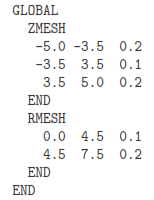
The axial specification states that the initial triangular element base (before smoothing and fitting) is 0.2 cm in the zones -5.0 cm ≤ z ≤ -3.5 cm and 3.5 cm ≤ z ≤ 5.0 and 0.1 cm near the coil. Figure 31 shows the result. Note that Mesh has fitted the coil boundaries exactly and made smooth transitions between regions of different element sizes.
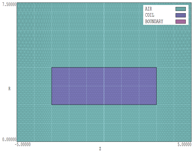
Figure 31: Variable resolution mesh for the magnet coil solution.
To make useful comparisons of the numerical results, we need a baseline. The theoretical expression5 for the on-axis field at the midplane of a solenoid (z = 0.0 cm, r = 0.0 cm) with finite length and radial thickness is:
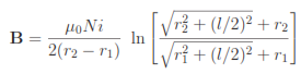
For the values Ni = 2500.0, r1 = 0.02 m, r2 = 0.04 m and l = 0.06 m, Eq. 5 yields the value Bz(0, 0) = 0.037186 tesla.
For the study, we will expand the boundaries (keeping rmax = 1.5zmax) and compare the value of Bz(0, 0) to the infinite-space result. We will use the following nine values for zmax: 5.0 cm, 6.0 cm, 7.0 cm, 8.0 cm, 9.0 cm, 10.0 cm, 12.50 cm, 15.0 cm and 20.0 cm. We could do each calculation interactively: create nine mesh scripts, run and analyze nine PerMag solutions. That’s the hard way. Field Precision programs offer a useful option for extended calculations. Batch files and external programs (e.g. python scripts) can not only run the technical programs, but they can also control how the program interprets variable quantities in the input script. In the present application, the Mesh input script is modified to the following form:
5 http://www.netdenizen.com/emagnet/solenoids/solenoidonaxis.htm.