![]()
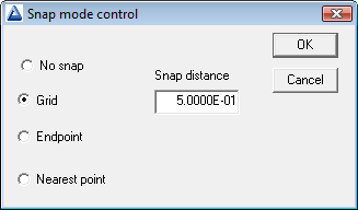
Figure 33: Set snap mode dialog of the Mesh drawing editor.
9 Magnetostatic solution: the role of steel
To complete our study of the solenoid coil, we’ll proceed to a practical design by adding a magnet-steel shield. Here, the term magnet-steel designates a soft material with high relative permeability. The term soft means that the steel has a narrow hysteresis curve and has negligible permanent magnetization. Magnet-steel serves three functions in an electromagnet:
1. High-µ materials act as conductors of magnetic flux with little expenditure of energy. The use of atomic currents of materials to carry the return flux of a magnet means that the real currents in the drive coil can be reduced.
2. Ferromagnetic materials act as shields. Return flux prefers to flow through the steel, reducing the fringing fields of the magnet.
3. The magnetic flux density B is constrained to point almost normal to the surface of a material with µr ≫ 1.0. Some control may be exerted over field variations by shaping the surfaces of the steel.
The example will demonstrate these effects. The underlying assumption is that the fields generated by drive coils are low enough so that the ferromagnetic material is not driven into saturation. The next article discusses the nature of saturation effects and how to model them.
We’ll start with the magnetic solution for a bare cylindrical coil discussed in the previous chapter with boundaries zmin = −6.0 cm, zmax = 6.0 cm and rmax = 9.0 cm. We’ll add an additional region to the input script BareCoil.MIN to represent the external iron shield using the Mesh Drawing Editor. Run tc.exe, set the Data folder to the working location and launch Mesh. Use the command File/Load/Load script (MIN) and choose BareCoil.MIN. Then, use the command Edit script/Edit script (graphics) to open the drawing editor. The vectors for the three regions are displayed and current region is set to 3. Click the Start next region tool. We will add vectors to represent the outline of the shield to Region 4. Click the Set snap mode tool to open the dialog of Fig. 33. For convenience, we specify that entered points will snap to the drawing coordinate system with a resolution of 0.5 cm.
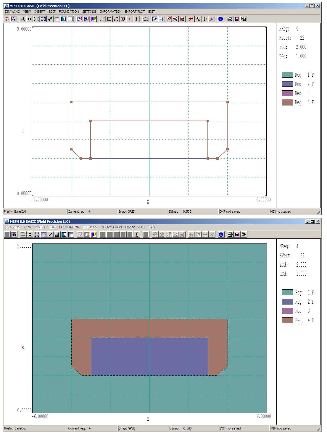
Figure 34: Top: adding a region in the Mesh Drawing Editor. Bottom: checking the fill status.
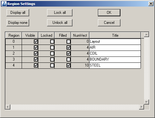
Figure 35: Region properties dialog in the Mesh Drawing Editor.
Click on the Line tool to enter a series of vectors that outline the shape shown in Fig. 34 (brown lines). In the line entry mode, move the cursor to snapped locations and left-click on the start and end points of each of the ten vectors. Be sure that they all connect and define a closed shape. Snap mode helps to ensure that the end point of one vector connects exactly to the start point of the next. When you have finished the last vector, right-click the mouse to exit the line entry mode.
Choose the command Settings/Region properties to open the dialog of Fig.35. Give the new region the name Steel and check the Filled box (we want to assign a high value of µr to all the enclosed elements). Exit the dialog. To confirm that the vectors of the new region constitute a connected and closed set, click the Toggle fill display command. The lower display of Fig. 34 shows valid filled regions.
Finally, it is a good practice in electrostatic and magnetostatic solutions to group regions with fixed boundary conditions (electrostatic potential or vector potential) at the end of the Mesh script. Choose the command Settings/Region order. Check the box for Steel and then click the Move UP button. Click OK to exit the dialog. To conclude. click the Export MIN tool and save the revised data as the file SteelShield.MIN. Exit the drawing editor. Click the Load script (MIN) tool and load the new script. Process the mesh and then click the Save mesh (MOU) tool to create the file SteelShield.MOU.
Run PerMag, click the 1 tool and choose the new mesh file. The dialog is similar to the previous example, except for the new region. Fill in the values as shown in Fig. 36. Save the file as SteelShield.PIN and then run a solution. To make a comparison, we need a solution without the steel. Here’s a quick way to create it. Choose the command File/Edit files and pick SteelShield.PIN. Comment out the specification for high µr (put an asterisk at the beginning of the line) and replace it with the value for air:
* Mu(3) = 5.0000E+02
Mu(3) = 1.00
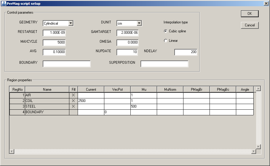
Figure 36: Dialog to set up the PerMag solution.
Save the result as NoShield.PIN and exit the editor. Then generate an additional PerMag solution.
We can find out a lot about the effect of steel just by looking at a plot of lines of magnetic flux density B (Fig. 37). With no steel shield, the lines spread out over the entire external region and the solution is strongly influenced by the boundaries. With the shield, the return flux lines are conducted through the steel. In this case, fringing fields are small and the boundaries have almost no effect on the solution. As expected, lines of B entering and exiting the steel are normal to the surface. The shield also contains lines axially and |B| is more uniform within the coil.
For a quantitative comparison, we can inspect scans of magnetic flux density along the axis, Bz(z, 0). Prepare and run the following analysis script:
NScan = 100
Output Shield_Analysis.DAT
Input NoShield.POU
Scan -6.0 0.0 6.0 0.0
Input SteelShield.POU
Scan -6.0 0.0 6.0 0.0
EndFile
Fig. 38 shows plots of computed values. The shield does improve axial containment of magnetic flux. A significant result is that field magnitude inside the coil (e.g., the working volume of a magnetic lens) is 38% higher. Note that the two solutions have the same coil cross section and NI product. Alternatively, suppose the goal is to achieve a given central value Bz(0, 0). The result of Fig. 38 indicates that the required NI product with the shield is only 73% that for the air coil, so the drive power would be cut almost in half. This effect arises because the coil need not supply field energy to support the return flux.
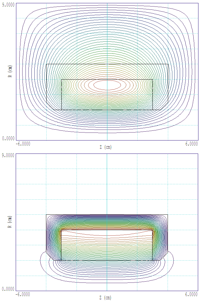
Figure 37: Lines of magnetic flux density B. Top: No shield. Bottom: With shield.
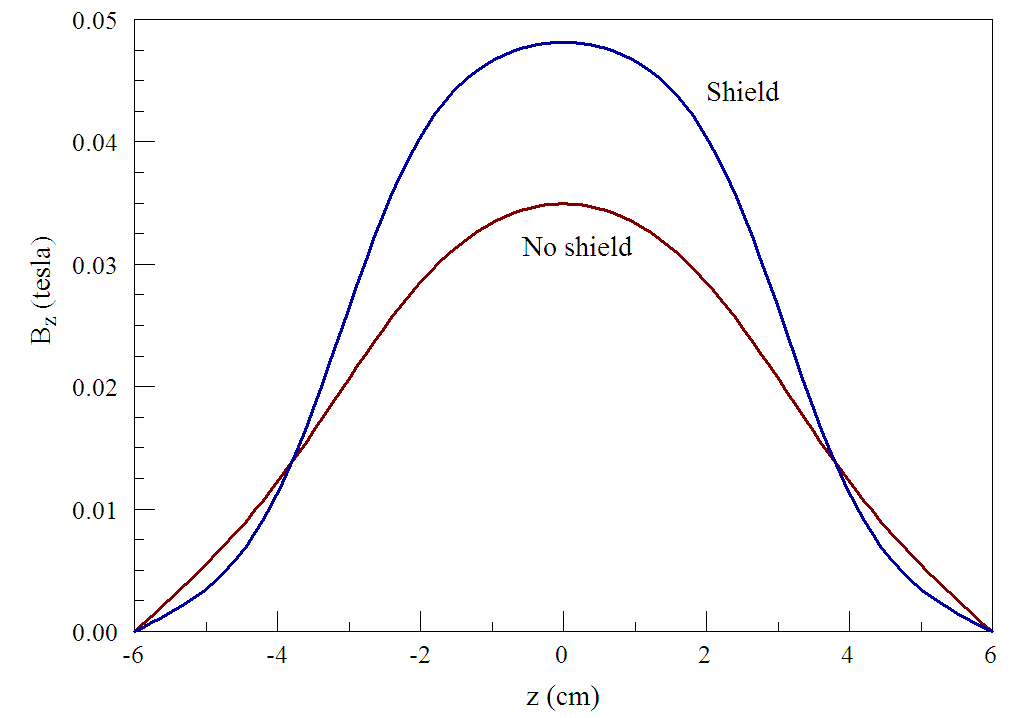
Figure 38: Scans of Bz(z, 0) with and without the shield.
The condition of a fixed value of µr applies if the atomic currents in the iron are proportional to the drive currents in the coil (i.e., the hysteresis curve approximates a straight line). Some- times, the hysteresis curve may have a more complex variation. Even more important, there is a maximum value of atomic current in the material equivalent to alignment of all magnetic domains. At some value of coil current, the proportionality can no longer hold. The effect is called saturation of the magnetic material. The next chapter discusses how the non-linear effect of saturation is represented in PerMag.