![]()
10 Magnetostatic solution: when steel gets complicated
Complex material behavior is the main reason why magnetostatic solutions are generally more difficult than electrostatic solutions. Usually, dielectrics can be characterized by a single value of the relative dielectric constant ǫr up to the point where they break down. On the other hand, magnetic materials do unusual things even at normal values of flux density B:
• Magnet steels may exhibit variations of µr, with a drop to µr = 1.0 at higher field levels (saturation).
• In permanent magnets, the domains are locked in place, almost independent of the applied field.
We’ll talk about how to model permanent magnets in the next chapter. Here, we’ll concentrate on non-linear magnetic materials.
First, some definitions. The quantity B0 is the magnetic flux density at a point in space created by coils or permanent magnets. We’ll call it the applied flux density. In the absence of steel, the total flux density is given by B = B0. In the PerMag program, the relative magnetic permeability of isotropic materials is defined as µr = |B|/|B0|. Therefore, µr = 1.0 in air or vacuum. In steel, the alignment of domains creates a material flux density that adds to the applied flux density. Therefore, µr is greater than 1.0. As we saw in the previous article, the utility of steel follows from that fact that µr ≫ 1.0.
Magnetic materials are characterized by curves of the form |B| versus |B0| (or |B| versus |H|, where H = B0/µ0). If the variation is a straight line, then µr = constant and we say that the material is linear. Magnetic materials may exhibit linear behavior at low fields, but they always become non-linear at high fields (a few tesla). Equivalently, we can characterize materials with a plot of |B| versus µr. Figure 39 shows such a plot for steel 1020, a common material for magnet cores. At low |B|, the value of µr is much greater than unity and changes considerably (i.e., the |B|-|B0| curve is not a straight line). Physically, the curve implies that it takes some pushing to start aligning domains but things get easier when they begin to come around.
The notable feature of the curve is that µr approaches 1.0 when all the domains are aligned. In this case, the material contribution to B does not get higher as B0 increases, so that B → B0. The saturation flux density corresponds to the point where all domains become aligned. For steel 1020, the value is Bs = 1.75 tesla. PerMag can perform self-consistent calculations for non-linear materials using |B|-µr data . PerMag simultaneously adjusts the value of µr in elements based on the current value of |B| as it performs the iterative matrix solution of the finite-element equations.
Let’s work on some calculations. The first question is whether the variations of µr below saturation will make a significant difference in the calculation. In other words, do we need to worry about getting the |B|-µr curve exactly right? To illustrate, we’ll use the example of the H magnet illustrated in Fig. 40. It has a planar rather than cylindrical geometry. Here, there are variations in x-y but the steel core and coils extend an infinite distance in z. Such a
6The values of Fig. 39 are used as PerMag input for the calculations of this chapter
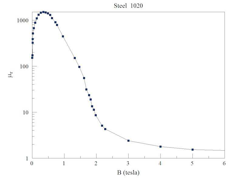
Figure 39: Plot of relative magnetic permeability versus |B| for Steel 1020.
calculation is often a good approximation to the central section of a long dipole magnet. Both sets of coils produce a upward-directed flux that is conducted by the steel to the air gap, the working volume.
To start, we’ll address the question: how does the value of µr in the core affect the field distribution? We’ll use the command-line parameter method discussed in Chap. 8, assigning fixed µr values over the range 5.0 to 10,000 and comparing values |B| in the air gap. Before beginning, its useful to recognize that the solution of Fig. 40 involves more work than is nec- essary. The fields in the four quadrants are mirror images. As an alternative, we could find the solution only in the first quadrant by applying appropriate symmetry conditions along the boundaries x = 0.0 and y = 0.0. Lines of B are normal to the boundary at y = 0.0. Here, we could apply the Neumann condition (the natural condition for a finite-element solution). Lines of B are parallel to the other three boundaries, implemented by the Dirichlet condition Az = 0.0.
Figure 41 shows a plot of By in the magnet air gap at the midplane (0.0,0.0) and edge (2.0,0.0) of the magnet gap as a function of µr. The relative magnetic permeability has a strong influence at low values but little effect for large values. We can understand what’s happening by inspecting Fig. 42, a plot of lines of B. The top illustration shows a solution with high µr. In the case, the low-reluctance core carries most of the flux, which flows up between the coils and returns across the air gap. A small fraction takes a short-cut around the outside of the outer coil (leakage flux). The reluctance of the air gap causes the flux to spread out to increase the cross-section area (fringing flux). Note that the lines of B entering and exiting the core are almost normal to the surface. In contrast, the lower illustration shows the case with low µr. In this case, the core has a high reluctance, increasing the leakage flux. A reduced fraction
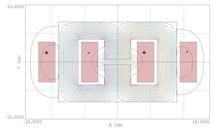
Figure 40: Geometry and calculated lines of B in the cross section of an H magnet.
of the flux is transported to the air gap, hence the reduced value of By. Finally, we’ll consider why there is little change in the solution when µr changes by a factor of 10 between 1000 and 100000. The important quantity in a finite-element magnetic field calculations is not µr, but actually γ = 1.0/µr. A value γ = 1.0 represents air, and a value γ → 0.0 is characteristic of unsaturated steel or iron. Both 1/1000 and 1/10000 are close to zero, so the change in µr makes little change in the solution.
We’ll conclude with a full non-linear calculation for the H magnet. Table 2 shows the script HMagnet.PIN that controls the PerMag calculation. Region 2 is the steel core. Instead of assigning a fixed value, the code reads the table of information plotted in Fig. 39. The coils are set up for two calculations at high and low current. The values of drive current were chosen for solutions such that the core steel is well below and well above saturation.
Because the two processes of the material adjustment and the iterative matrix solution are performed simultaneously, program controls must be optimized to ensure convergence. Some experimentation may be necessary. Consider the following commands:
MaxCycle = 8000
Avg = 0.05
Update = 20 500
The quantity MaxCycle is the maximum number of matrix iterations, set to a fairly high value. The quantity Avg controls averaging of µr values between cycles. The low value is used to avoid oscillations of µr. Finally, the Update command states that µr should be recalculated every 20 iteration cycles and that the program should wait 500 cycles before corrections to ensure a good starting solution.
Figure 43 shows the variation of µr at low and high current. At low current (upper solution), the relative permeability exceeds 1000 over most of the core volume. The low values at the top reflect the fact that |B| is small and the elements are on the left-hand side of the curve of
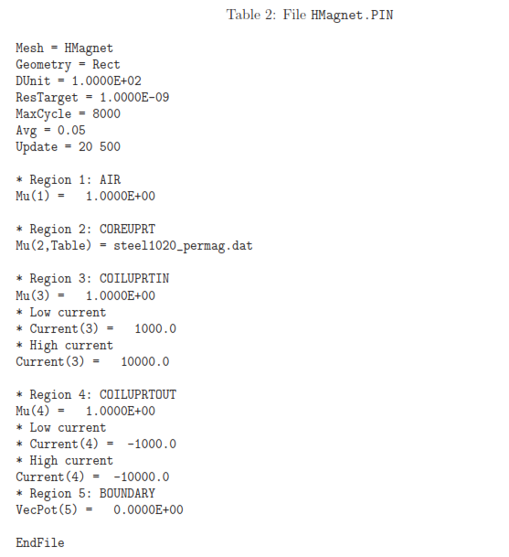
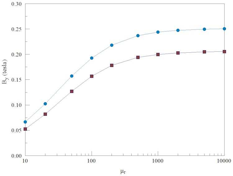
Figure 41: Variation of By(0, 0) [blue] and By(2, 0) [red] in the H magnet as a function of relative magnetic permeability in the steel core.
Fig. 39. An inspection of lines of B in Fig. 44 (top) shows that they are contained mainly in the core. Lines outside the core are normal to the surface. The midplane field is By(0, 0) = 0.2459 tesla. At high current (Fig. 44 bottom), many regions of the core are driven into saturation, particularly the vertical piece adjacent to the air gap. The figure shows enhanced fringing flux near the air gap. The central field value is By(0.0) = 1.484, only 6.03 times the field at one tenth the drive current. Note that the field lines near the air gap are not normal to the core surfaces, affecting the profile of B across the gap.
In summary, we addressed the following issues in this chapter:
• Typical variations of µr for soft magnetic materials.
• Physical implications of the magnitude of µr, particularly as it affects the reluctance of steel structures in magnets.
• Procedures to set up and to interpret non-linear solutions in PerMag.
The next article will discuss how permanent magnets work and how to build solutions for 2D permanent magnet devices.
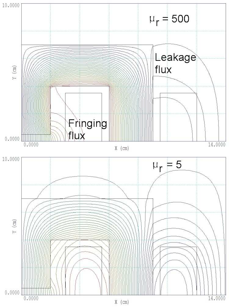
Figure 42: Lines of B at high and low values of relative magnetic permeability.
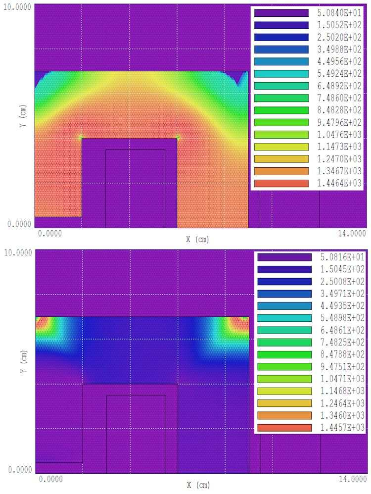
Figure 43: Spatial variation of relative magnetic permeability in the H magnet solution for low (top) and high (bottom) drive currents.
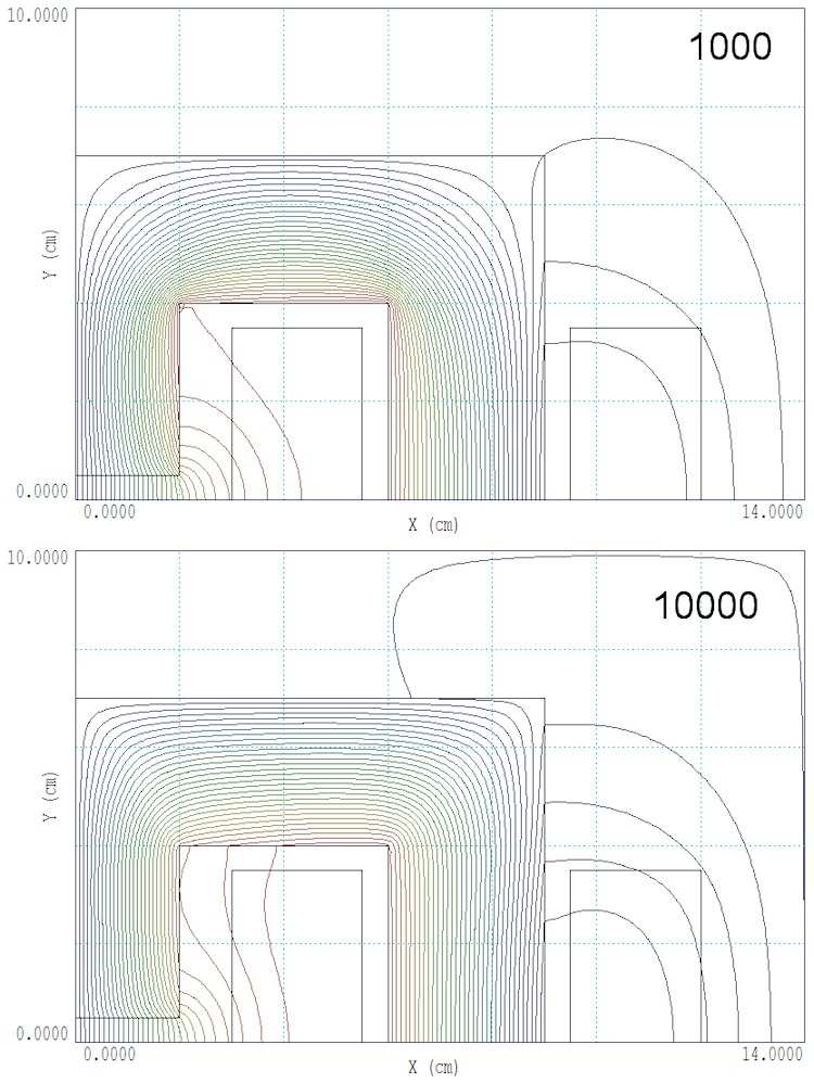
Figure 44: Lines of B in the H magnet solution for low (top) and high (bottom) drive currents.