![]()
11 Magnetostatic solution: permanent magnets
As the final topic in two-dimensional magnetostatics, we’ll consider solutions with permanent magnets. To start, it’s useful to review how permanent magnets work. Introductory elec- tromagnetic texts sometimes don’t treat the topic, and the explanations in many specialized references are overly complex.
The electrons of many atoms carry a circulating current, like a small current loop. Such an atom has a magnetic moment. The magnetic moment is a vector pointing from the center of the loop normal to the current. It points in the direction of the magnetic flux density B created by the loop. The distinguishing feature of ferromagnetic materials is that the atoms prefer to orient the currents in the same direction (a quantum mechanical effect). A region where all atoms are aligned is called a domain. The upper section of Fig. 45 shows the summation of aligned atomic currents in a domain. Currents on the inside cancel each, so the net result is a surface current in the direction normal to the magnetic moment.
In the natural state of a ferromagnetic material, the orientation of domains is randomized so that there is no macroscopic field outside the material (bottom section of Fig. 45). To generate such a field would require energy. Let’s say that we supplied the energy by placing the material inside a strong magnet coil. In this case, the domains line up and the current of all domains sum up as in the top section of Fig. 45. The domain currents cancel inside, but there is a net surface current on the object. If we turn off the coil, the domains of a soft magnetic material return to a random distribution. On the other hand, suppose we could physically lock the domains in position before we turned off the coil. In such a hard material, the object retains its surface current and can generate external fields. The energy for the field was supplied by the magnetizing coil and it was bound in the material. Such a object is called a permanent magnet.
The distinguishing feature of modern permanent magnet materials like neodymium-iron and samarium-cobalt is that domain locking is extremely strong. The domains remain lined up, independent of external processes. This property makes it simple to model the materials. Let’s review some definitions and facts. The direction of the magnetic moments of the aligned atoms (and domains) is called the magnetization direction. Suppose we have a permanent magnet that is long along the direction of magnetization and self-connected (e.g. a large torus). In this case, there is no external field and the flux density inside the material is generated entirely by the surface currents. This intrinsic flux density is called the remanence flux, Br, the most important quantity for characterizing a permanent magnet. A typical value for neodymium iron is Br = 1.6 tesla.
We can express the surface current density in terms of the remanence flux. Take Br as a vector pointing along the direction of magnetization and let ns be a vector normal to the surface of the permanent magnet. The surface current density is given by
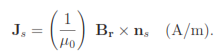
We can use PerMag to confirm this physical interpretation. The top section of Fig. 46 shows a calculation in cylindrical geometry for an annular permanent magnet in space (i.e., no iron, coils or other permanent magnets). The remanance field is Br = 1.5 tesla and the direction of magnetization is along z. The plot shows lines of B. According to the interpretation of Fig. 45,
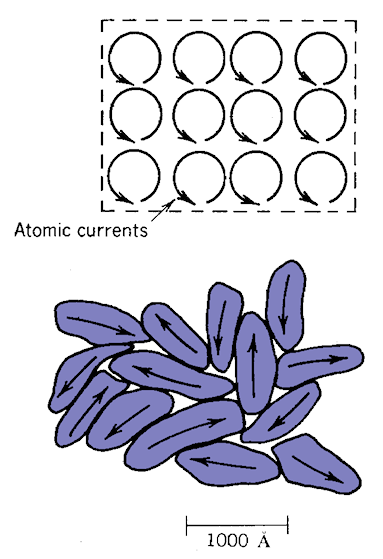
Figure 45: Top: alignment of atomic currents in a domain. Bottom: alignment of domains in unmagnetized material.
we would get the same results by replacing the permanent magnet with thin surface current layers. Equation 6 implies that there should be no current on the ends and uniform current density Js = 1.193 MA/m on the inner and outer radial surfaces. In the second model (bottom section of Fig. 46), the permanent magnet is replaced by two thin solenoid coils (length = 0.08 6 m, thickness = 0.00125 m). The total current of the outer coil is (1.193 × 10 )(0.08) = 95470.0 A and the current on the inner coil is -95470.0 A. The lower section of Fig. 46 shows that the calculated lines of B are indistinguishable from the permanent magnet calculation. For a quantitative check, we can compare scans of Bz along the axis. Figure 47 shows the results. There small difference is a result of the finite thickness of the surface current layer.
If permanent magnets are that simple, where could confusion arise? Unfortunately, things are more challenging when we talk about older materials like Alnico. Such materials are char- acterized by a demagnetization curve. Typically, the curve is a plot of |B| inside the permanent magnet versus |H|. Here, |H| is the applied magnetic field that arises from coils and other permanent magnets. It is easier to see the meaning of the curve if we make the plot in terms of the applied magnetic flux density, B0 = µ0H. Applied fields have no effect on a modern material. Therefore, the total flux density inside the material is simply
B = Br − B0. (7)
Figure 48a shows a plot. The value of applied magnetic field when B = 0.0 is called the coercive force Hc. For modern materials, the coercive force is
 . (8)
. (8)
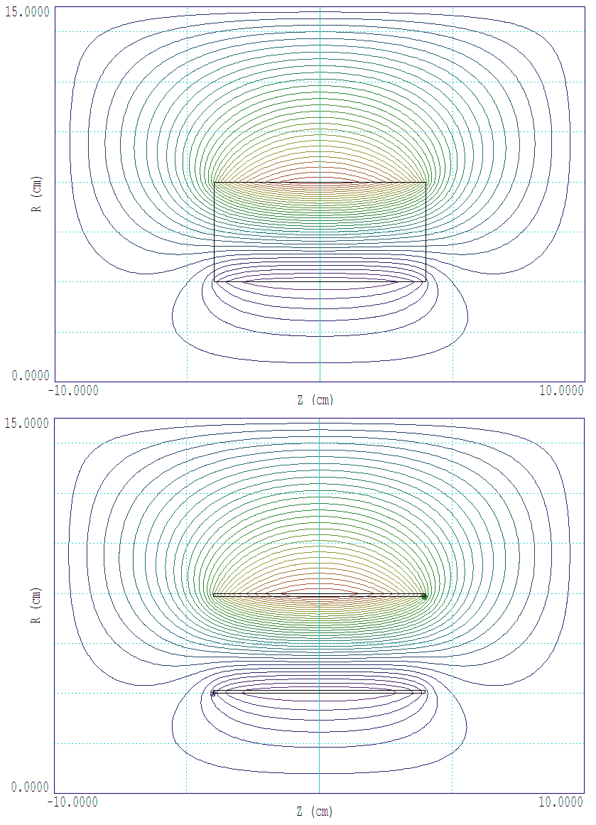
Figure 46: Lines of magnetic flux density for an annular permanent magnet (top) versus equivalent surface current layers (bottom).
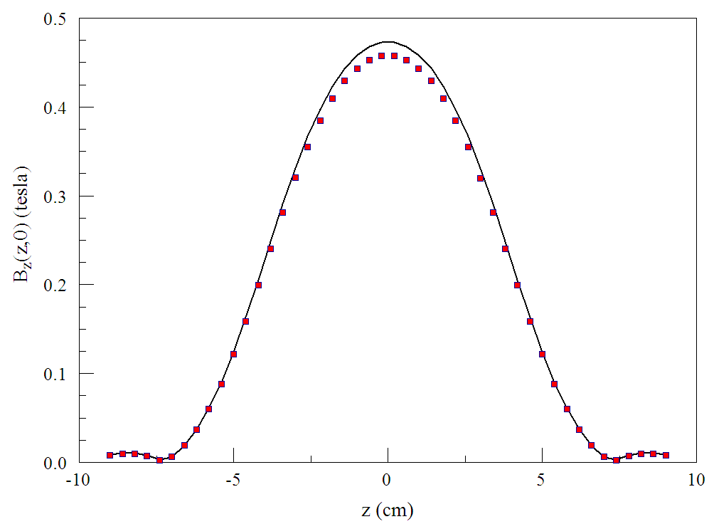
Figure 47: Scans of By(x, 0) for an annular permanent magnet versus equivalent surface current layers.
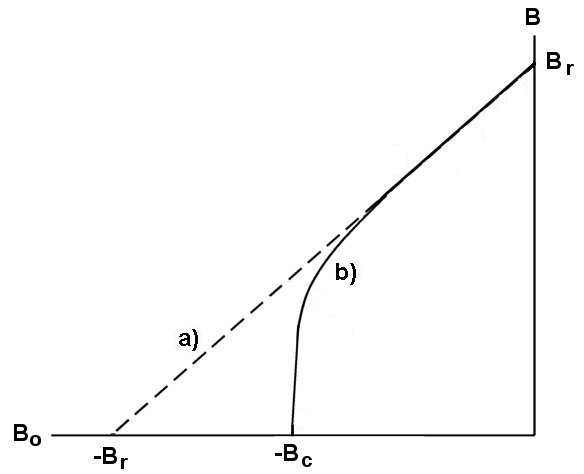
Figure 48: Demagnetization curves for modern (a) and older (b) permanent magnet materials.
It is clear that neither the demagnetization curve or the coercive force are particularly meaningful for materials like NdFeB. On the other hand, the concepts are useful for older materials. Here, the domains are not tightly locked. Putting such a magnet in a device with an air gap could cause degradation of the alignment so that the total flux density falls below the ideal curve (Fig. 48b). PerMag can solve such problems, but it is important to clarify what the solutions mean. Suppose you bought an Alnico magnet magnetized at the factory and shipped with an iron flux return clamp (i.e., B = Br). If you could move it instantaneously to the application device, then the operating point calculated by PerMag would apply. On the other hand, if you removed the clamp so the permanent magnet was exposed to an air gap and possibly dropped it on the floor, then the material would have undergone an irreversible degradation and the fields generated will be lower than predicted. The best way to get the predicted performance based on the demagnetization curve is to magnetize the material in situ. One big advantage of modern materials (beside their strength) is that they achieve the predicted performance, even if they are magnetized at the factory, shipped from China and moved to the assembly.
We’ll conclude with an application calculation, a bending magnet for an ion spectrometer. It is a long assembly, so we will do a preliminary 2D calculation in a cross section. The top section of Fig. 49 shows half the geometry (there is a symmetry plane with Neumann boundaries at y = 0.0 cm). The goal is to create a dipole field By in the air gap to bend ions in the x direction. The arrow shows the magnetization direction of the permanent magnet (NdFeB with Br = 1.6 tesla). Two features ensure the maximum air-gap field for the given magnet surface currents:
• A steel core carries the return flux.
• The permanent magnet is placed close to the gap.
The figure shows the calculated lines of B. Figure 50 shows a scan of By along x across the air gap. The field is strong but non-uniform, probably of little use in a spectrometer. To correct things, we can take advantage of one of the properties of soft steel, field shaping. Consider the effect of adding a steel layer adjacent to the gap. The lower section of Fig. 49 shows the change in lines of B. The steel shifts flux away from the center to the edges of the gap. Figure 50 shows the effect on the field scan. With some sacrifice in the magnitude of the flux, steel shaper gives a working volume of approximately uniform field.
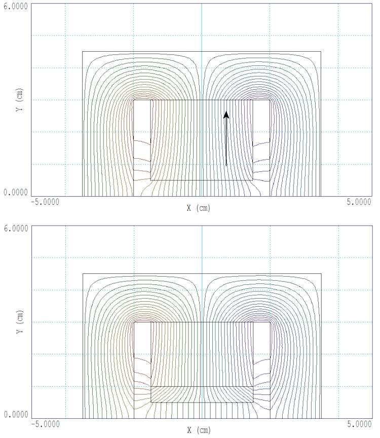
Figure 49: Application example, permanent-magnet ion spectrometer. Top: bare magnet. Bottom: magnet with steel insert for field shaping.
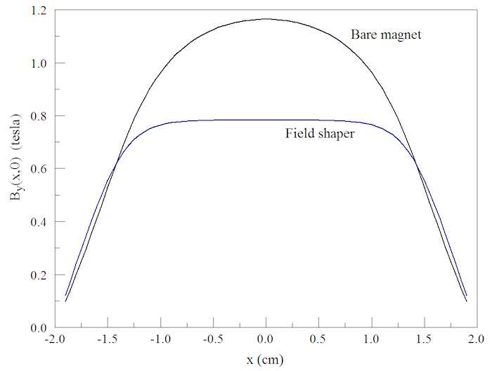
Figure 50: Spectrometer application, scan of By(x, 0) with and without the steel insert.