![]()
13 3D electrostatic example: STL input
To introduce a 3D calculation, well step through a complete field solution for a sophisticated electron gun designed at the Lawrence Livermore National Laboratory to generate sheet beams. We’ll use prepared input files - following chapters will help you prepare you own inputs.
To start, run the AMaze program launcher and set the Data folder to point to a working directory. Copy the following files supplied in the example archive to the working directory:
sheetbeam.min
sheetbeam.hin
cathode.stl
focus.stl
output.stl
The text file sheetbeam.min is a set of instructions to MetaMesh defining the shapes and assembly method of the gun parts. The instructions were built in the interactive environment of Geometer. The text file sheetbeam.hin gives HiPhi the material properties and other pa- rameters needed to generate a finite-element solution. The stereolithography files cathode.stl, focus.stl and output.stl were supplied by a laboratory engineer who exported them from a Solidworks model. They define shapes that are too complex to create from a summation of simple solids.
As we saw in Chap. 6, the procedure for 2D shapes is relatively simple. Objects are created from a boundary outline of line and arc vectors. The outlines may be derived from or exported to DXF files. In contrast, shapes encountered in the 3D world may be much more complex. A flexible approach is essential to make the task manageable. The following principles underlie the operation of Geometer and MetaMesh. Their implications will become clear as we move through the example:
• Objects (like electrodes and dielectrics) are constructed from one or more Parts.
• Physical properties (like potential and relative dielectric constant) are assigned to Regions. Each Part belongs to a Region.
• An object may be constructed from several parts associated with the same region. For example, a grounded electrode could be composed of parts that belong to a region with fixed potential 0.0 V.
• Parts are processed in the order in which they appear in the MetaMesh input file. The currently-processed part overwrites any shared volumes with previously-processed parts.
Parts are defined at a standard position and orientation. They may be moved or rotated to a final configuration in the solution space.
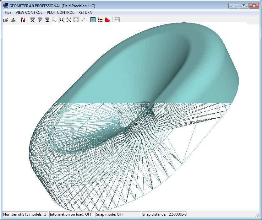
Figure 53: Geometer STL viewer, showing solid and wireframe views of focus.stl.
Its clear that the idea of a part is central to the mesh building process. There are two types:
• Parametric models for simple shapes like cones or spheres. These models are built into Geometer and MetaMesh and do not require external data.
• Arbitrary shapes created with 3D CAD programs like SolidWorks and exported as files in the STL format. These files must be loaded into Geometer or MetaMesh.
A mesh may combine both types of parts.
Lets get started with the calculation. To begin, its useful to understand the informa- tion in STL files. Run Geometer and click the STL viewer command. The program be- comes a full-featured viewer that can display the shapes defined by individual STL files and their relationships in space. Click File/Add model and choose focus.stl. Click View con- trol/Orthogonal/perspective to enter the 3D mode. This is an interactive environment based on OpenGL. Move the mouse cursor to the sides and left click to change the view. You can also move the cursor toward the center and left or right-click to zoom in or out. The view looks like the right-hand side of Fig. 53. The part is a dish-shaped focusing electrode with a hole for the cathode.
To see the inherent data of the STL file, click Plot control/Model display. Uncheck the Solid box to create a view like the left-hand side of Fig.53. The view shows the set of contiguous triangular facets that define the surface of the part. The STL file is simply a list of facets. The facets shown are typical of those created by 3D CAD programs. Although all facets
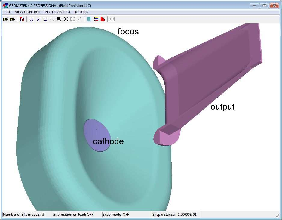
Figure 54: Full set of STL shapes for the assembly.
are theoretically correct, they may vary considerably in scale. To determine if an element is inside an STL shape, MetaMesh must analyze all facets, an intensive activity where parallel processing is a big advantage.
Return to a solid view of the surface and load the other two parts to get a view like that of Fig. 54. The engineer exported the parts from a SolidWorks assembly. In this case, the coordinates of facets in the STL file are absolute with respect to the assembly space rather than relative to the part. Therefore, the facets not only define the shape of parts, but also their positions and orientations relative to each other7.
The parts as loaded define the full volumes of the cathode and focus electrode, but only half of the output transport tube. This is not a problem because by symmetry it’s sufficient to perform a calculation only in the first quadrant of the x-y plane. MetaMesh automatically clips over-sized parts. There is one problem that you can see by shifting to the Orthogonal view and clicking View control/Y normal axis. The Solidworks model corresponds to a beam moving in the -z direction. For transport calculations, we want the beam to move in +z following the standard convention. The modification will be made during MetaMesh processing.
Exit Geometer and run MetaMesh. Click File/Load MIN file and choose sheetgun.min. Click the Process mesh command and wait for the program to complete its analysis. It takes about 20 seconds on a multi-core computer to generate a mesh with 1.3 million elements. Right-click to close the messages. Choose Plot3D to observe the display of Fig. 55. The plot
7Note that we could move the parts to different positions by adding shift operations in Geometer.
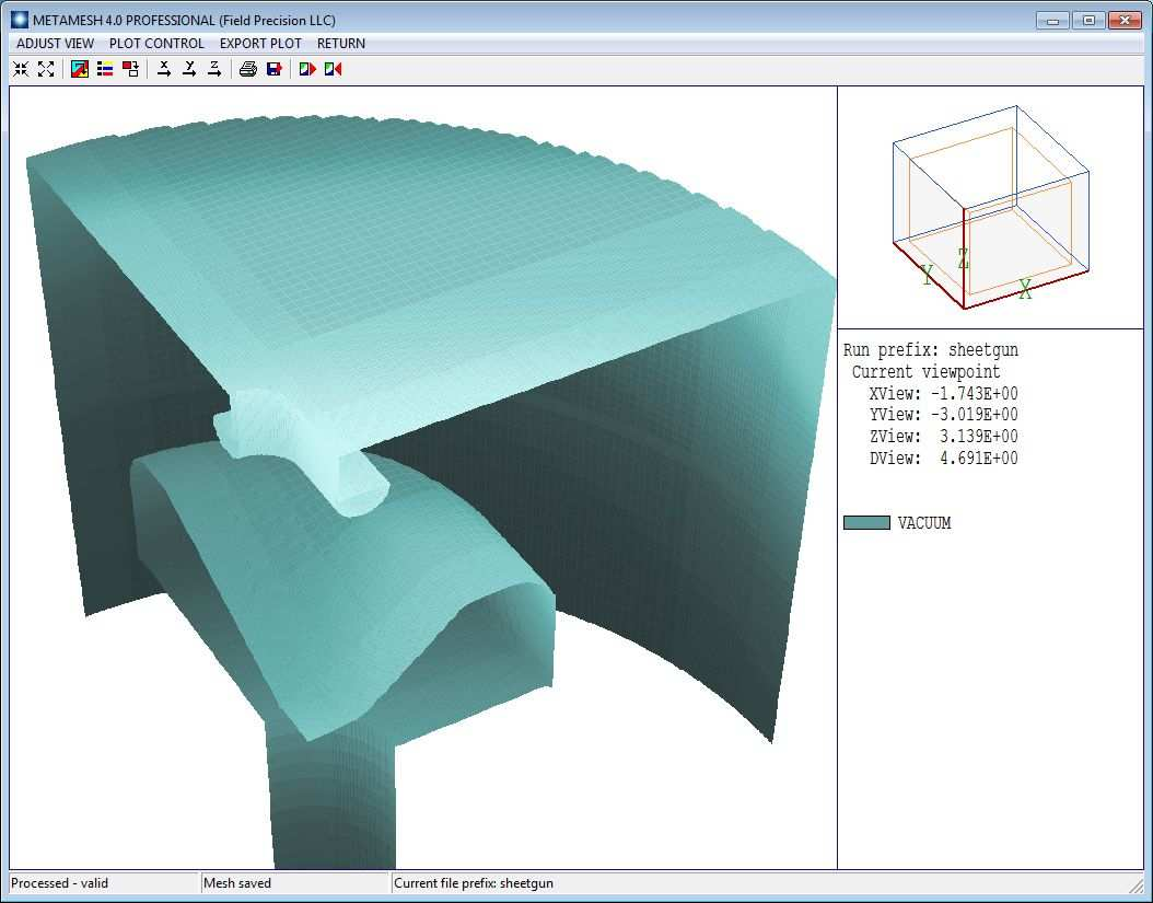
Figure 55: Completed mesh, outline of the vacuum region.
of the surfaces of elements of the vacuum region) indicates a good representation of all the electrodes. The parts defined by STL files are present, but much more has happened. The mesh has been created in the first quadrant with fine resolution of the cathode surface, the hexahedron elements conform closely to the theoretical shapes, the beam direction points in +z, the assembly is inside a cylindrical vacuum chamber and there is a support rod for the cathode. All will be explained in the next chapter where we take a close look at the MetaMesh script.