![]()
14 3D electrostatic example: mesh generation and solution
In this chapter, we’ll conclude the example 3D electrostatic solution. The previous chapter introduced the concept of mesh Parts and Regions. The emphasis was on input from 3D CAD programs via STL files. Here, we’ll consider how MetaMesh uses the STL data and processes extra information to create the result of Fig. 55. We could go through all the interactive operations in Geometer to define the parts, but there’s a quicker way to understand the setup. The end result of Geometer activities is a MetaMesh input script that includes all the information. We’ll study the script directly. A following chapter shows how to use Geometer to create a solution from scratch.
Run AMaze and launch MetaMesh. We’ll assume that the Data folder is still point- ing to the working directory of the previous chapter. Click File/Load MIN file and choose sheetgun.min. Then click File/Edit MIN file to view the contents of the script. The first part of the Global section has detailed specifications for element sizes over multiple zones along the axes. The feature was necessary for accuracy in subsequent beam emission calculations – the details are not of immediate concern. Instead, we’ll concentrate on the part definitions shown in Fig. 568.
The parts named Anode, Focus and Cathode (marked in green) use the STL models that we previously discussed. The Type command of each part section lists the associated STL file. The Fab (fabrication) command defines fitting controls – default values are usually sufficient. Although the intent is build the mesh around the assembly positions of the STL parts, we do want to reverse the emission direction to +z. This is accomplished with the commands:
Rotate 180.0 0.0 0.0 XYZ
Each command rotates the coordinates of all facet nodes 180o about the x axis relative to the assembly origin. The commands
Surface Region VACUUM
instruct the code to adjust all element facets of the part adjacent to Vacuum elements to conform closely to the defined surface of the STL model.
The assembly is located inside a cylindrical vacuum chamber of radius 1.23” that extends from z = 0.0” to the boundary of the solution volume at z = -1.50”. For high speed, HiPhi uses a structured conformal mesh, where structured means that the elements are arranged like an apartment building. The term conformal means that the apartments are not necessarily right-angle boxes9. The solution volume of a structured mesh is always a box. To create the vacuum chamber, we’ll fill the entire volume with elements assigned to the fixed-potential region Ground (part VChamber) and then carve out a cylindrical volume of elements associated with the Vacuum region. The part ExitPort is a slot to accommodate the beam exit aperture. The final part (Support) is a cylindrical pipe attached to the cathode. Note that this part belongs
8The text display is from the ConText editor using syntax highlighting definitions that we supply with the software.
9The general term for a six-sided solid where facets may not be at right angles is a hexahedron.
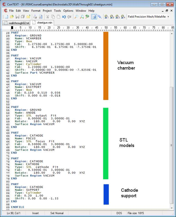
Figure 56: Part sections of the MetaMesh input script sheetgun.min.
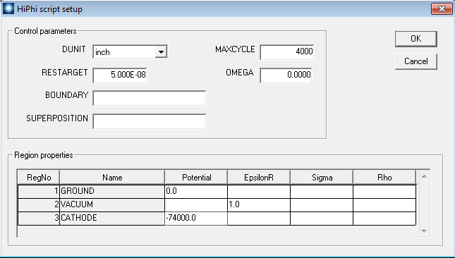
Figure 57: HiPhi dialog to set program parameters and the physical properties of regions.
to the same region as the cathode and the focus electrode. The physical property of the region in the HiPhi solution is is a fixed potential (-74.0 kV).
Exit the text editor and click the Process mesh command. MetaMesh reports progress of the mesh creation. When the program is finished, right-click to exit the report and use the File/Save mesh command to create the file sheetgun.mdf (Mesh Definition File).
We can now proceed to the HiPhi solution. Run the program, click Setup and choose sheetgun.mdf to open the dialog of Fig. 57. Fill in the values as shown. Click OK and save the results as sheetgun.hin. The resulting file has the contents:
Mesh = sheetgun
DUnit = 3.9370E+01
ResTarget = 5.0000E-08
MaxCycle = 4000
Parallel = 4
EndFile
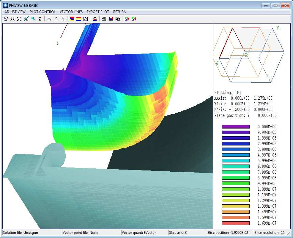
Figure 58: 3D plot of the assembly showing levels of |E| on the surface of the focus electrode.
The clean format of the file makes it easy to identify the functions of the commands. If you have the Pro version of HiPhi, the command
Parallel = 4
will reduce the run time.
Click the Run button and choose sheetgun.hin. The program generates a solution recorded as the binary file sheetgun.hou. We can get some useful information by checking the text listing files sheetgun.mls and sheetgun.hls created by MetaMesh and HiPhi. For example, the MetaMesh listing shows that the mesh contains 1,295,952 active elements10. The 4000 matrix- inversion cycles in HiPhi took 363 seconds to reach a relative residual11 of 8.6 × 10⁻⁷.
To complete the exercise, run PhiView and load sheetgun.hou. You can experiment with the options for 2D and 3D plots. Figure 4 shows an example, an overview of the levels of |E| on the focus-electrode surface. The red areas correspond to |E| = 16.7 MV/m.
10The term active means that the elements are not part of a fixed-potential region.
11The relative residual, a measure of the accuracy of the iterative solution, should be much smaller than unity.