![]()
15 3D electrostatic application: getting started
In this chapter we’ll advance to an application study, a concept for a capacitive position sensor. Rather than using prepared input files, we’ll build the entire solution from scratch. This chapter covers the initial steps in creating a 3D assembly with Geometer. Following articles will cover mesh generation, the finite-element solution and analysis techniques. The example emphasizes the internal parametric models of Geometer and MetaMesh rather than the STL models discussed in Chap. 13.
Figure 59 shows a view of the detector geometry. A dielectric object of known shape and size drops through the assembly along the y direction. A shaped drive electrode with an applied AC voltage creates a time-varying electric field that varies in the x direction. Changes in the mutual capacitance between the drive electrode and detector are sensed with a bridge network. The function of the detector is to confirm the presence of the object and its approximate position in x. The purpose of our calculation is find numerical values for the relative changes in mutual capacitance with the size and position of the object to gauge the accuracy requirements for the detector circuit.
Figure 60 gives an alternate 3D view of the assembly. For reference, we will use the following dimensions:
• The solution volume covers the region -2.50 cm ≤ x, y ≤ 2.50 cm and -0.25 cm ≤ z ≤ 3.00 cm.
• The metal case of thickness 0.25 cm encloses all sides of assembly except for a cut to house the detector and the upper boundary in z. We’ll discuss the physical meaning of this open boundary in a following article.
• The test object is a sphere of radius 0.375 cm.
• The detector is a rectangular plate with dimensions Wx = 1.75 cm, Wy = 3.25 cm and Wz = 0.25 cm.
• The cutout for the detector has dimensions Wx = 2.00 cm and Wy = 3.50 cm.
• The drive electrode is an extrusion of length Wy = 4.0 cm with a cross-section in the z-x plane defined by an outline of lines and arcs.
To start, decide on a working directory for the input/output files. Run the AMaze program launcher and point the Data folder to the directory. Run Geometer and click File/New script. In the opening dialog, enter the values shown in Fig. 61 to define the dimensions of the solution volume. When you click OK, Geometer automatically creates the first part12, a box that fills the solution volume. By default, the part is named SolutionVolume and is assigned to Region 1. The program displays a default orthogonal view in the x-y plane. The programs turns off the visibility of the first part because it would obscure the view of additional ones.
12see Chap. 13 for the definitions of parts and regions in Geometer
Figure 59: Detector geometry in the plane y = 0.0 cm.
Figure 60: 3D view of the detector assembly.
Figure 61: Dialog to start a new assembly in Geometer.
At this point, we need to make a strategy decision. We could associate the first part with air and add five parts to build up the metal case wall. On the other hand, it is easier to start with a block of metal that fills the solution volume and then to carve out an internal air volume. We’ll take this approach. To start, let’s define the physical regions that will be needed for the electrostatic solution and give them names that suggest their functions. Click Edit/Edit region names to bring up the dialog of Fig. 62. Replace the default region names with the ones shown and click OK.
Click the command Edit/Edit part, select SolutionVolume (the only one available) and click OK. The dialog on the left-hand side of Fig. 63 (left) shows the properties of the parametric model. The part is a Box that fills the solution volume. The box length in z is Wz = 3.25 cm.
The part has been shifted a distance 1.375 cm so that it fills the region -0.25 cm ≤ z ≤ 3.00 cm. Note that the name of the associated region has been changed to MetalWall. Change the default part name to MetalWall and then click OK to exit.
Next, we shall add a part that carves out the air volume. Choose Edit/Add part to open the model parameter dialog. Under Part type, choose Box from the popup menu. Set the Part name to Air and pick the Region Air. To leave metal walls of thickness 0.25 cm, the box should have lengths Lx = Ly = 4.50 cm and Lz = 3.00 cm. We need to set Zshift = 1.50 cm to fill in the region from 0.0 cm ≤ z ≤ 3.0 cm. The right-hand side of Fig. 63 shows the final state of the dialog. When you exit, the boundary of the air region appears in the plot. Click View/Y normal axis to check that the length and displacement of the box are correct. At this point, it’s a good idea save the work. Click File/Save script and accept the name DetectorStudy.MIN. The text file is in a format recognized as input to MetaMesh.
Figure 62: Dialog to define region names.
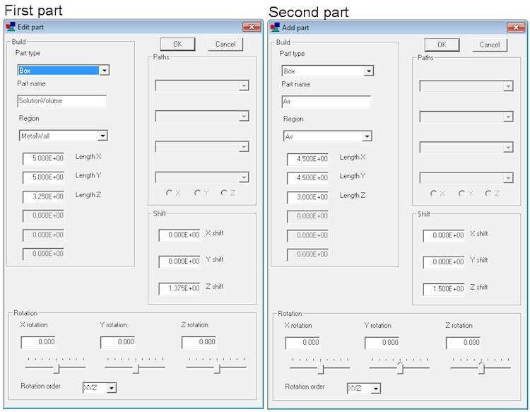
Figure 63: Edit part dialogs for the first (metal wall) and second (air volume) parts.
We need to include a slot in the wall to house the detector. Click on Edit/Add part and fill in the dialog with the following values
Type: Box
Part name: DetectorWell
Region: Air
Lx = 2.00
Ly = 3.50
Lz = 0.25
ZShift = -0.125
If everything is correct, the plot looks like Fig. 64. Go ahead and add the detector and the test object using the following parameters
Type: Box
Part name: Detector
Region: Detector
Lx = 1.75
Ly = 3.25
Lz = 0.25
ZShift = -0.125
Type: Sphere
Part name: Object
Region: Object
Radius = 0.375
ZShift = 0.625
The spherical object is centered at x = y = 0.0 cm with center 0.625 cm from the surface of the detector.
Viewing the state of the assembly requires some effort and experience. The surfaces of selected parts are plotted using OpenGL. When an encompassing part (like the metal wall) is included, it obscures internal parts. The following options are useful to display internal parts:
• Turn off the visibility of encompassing parts.
• Use a wireframe display for the encompassing part.
• Assign clipping planes to the part display.
The Geometer instruction manual gives a complete description of the plot controls. To illus- trate the current state of the setup, Fig. 7 shows a perspective view of the detector and object regions with the air region shown as a wireframe.
We need only define the drive electrode to complete the assembly. This part is an extrusion, a shape that extends a given distance along one direction with an arbitrary shape in the plane normal to that direction. In comparison, a turning is an arbitrary shape rotated about an axis of symmetry. In both cases, the shape is defined by a set of connected line and arc vectors. Extrusions and turnings are highly useful and versatile models that merit their own discussion. We’ll cover the topic in the next chapter.
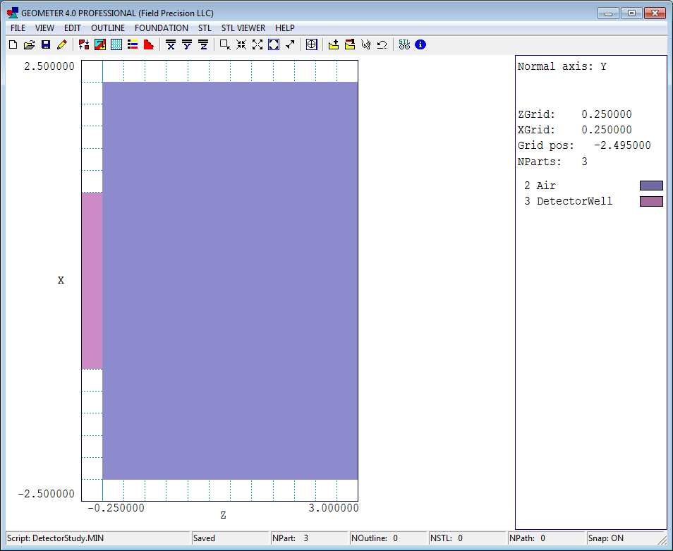
Figure 64: State of the assembly with the metal wall, air volume and detector slot.
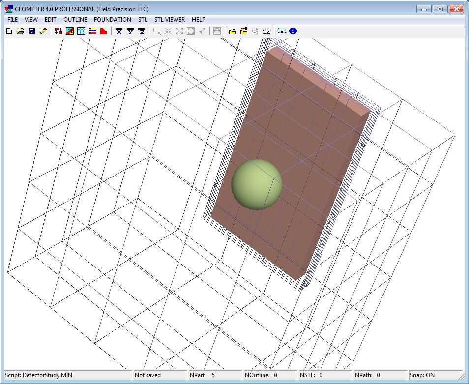
Figure 65: Perspective view of the assembly by regions with the air region shown as a wireframe.