![]()
16 3D electrostatic application: extrusions
In this chapter we’ll finish building the geometry of the capacitive detector and then generate a mesh. The remaining part is the drive electrode, an extrusion. Extrusions are the type of objects that you fabricate with a milling machine. They have arbitrary cross-section shapes that extend a specified distance along one direction.
A set of connected line and arc vectors defines the cross section of an extrusion. We call the set an outline. We already encountered outlines when discussing the 2D Mesh program in Chap. 4. The outlines in Geometer and MetaMesh have formats identical to those in Mesh – in fact, you can interchange them between the programs. One way to add an outline in Geometer is to construct it in the Mesh Drawing Editor (a full-featured CAD program) and then copy-and-paste the vectors. Geometer also has a built-in Outline Editor. It has many of the features of the Drawing Editor, but is designed for work on one outline at a time. In this article, we’ll concentrate on building outlines within Geometer.
First, a review of some concepts. Outlines are data sets available within Geometer that may (or may not) be used to define the cross section of one or more extrusions or turnings. In other words, outlines in the program exist independently of specific parts13. There are three ways to enter outlines in Geometer to make them available for part definitions:
• Copy-and-paste them from a Mesh script (New outline (Text) command).
• Load a MetaMesh input script (Load script command). The outlines of extrusions and turnings are stored and made available to construct additional parts.
• Draw them in the Outline Editor (New outline (Graphics) command).
We’ll concentrate on the third method. For reference, Fig. 66 shows the dimensions of the drive- electrode cross section. Although the following discussion refers to menu commands, there are entries in the toolbar for most of them.
Run Geometer and click File/Load script. Choose CapDetector.MIN, the file that contains the work from the previous chapter (the metal box and detector). Click Outline to open the Outline Editor. Choose New outline (Graphics) to open the dialog of Fig. 67. Supply the name DriveElectrode. The extrusion extends in the y direction in the assembly, so for convenience we will create cross-section vectors in the z-x plane. Check the ExtY radio button. For the View limits, enter the extreme dimensions of the outline as shown. Note that in a right- handed coordinate system normal to y, z corresponds to the horizontal direction and x to the vertical. When you click OK, Geometer opens the drawing editor with a view large enough to encompass the outline (Fig. 68).
We’ll enter the shape of Fig. 66 as a set of lines and then add the two fillets. Outline vectors must connect exactly, so it’s essential to use snap mode. By default, the program is set to Grid snap. There is an invisible grid of snap points beneath the displayed grid. The status line shows that the current snap grid distances are 0.1. We need to change the intervals so they are appropriate to the dimensions of Fig. 66. Click Draw/Grid control. In the dialog, uncheck Automatic intervals, set XGrid and YGrid equal to 0.25 and click OK.
13Geometer can store up to 80 outlines, each with up to 50 line and arc vectors.
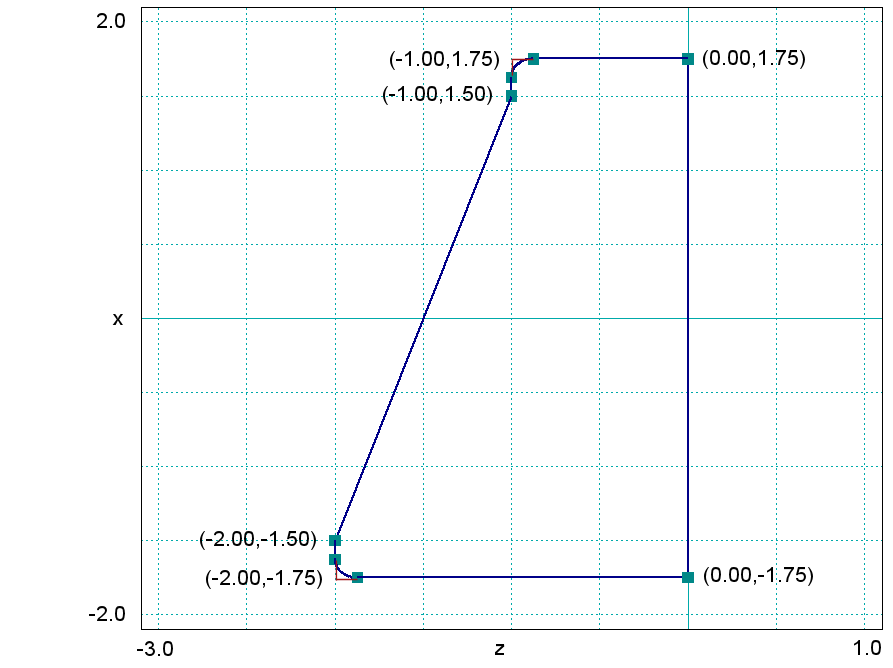
Figure 66: Geometry of the drive electrode cross section.
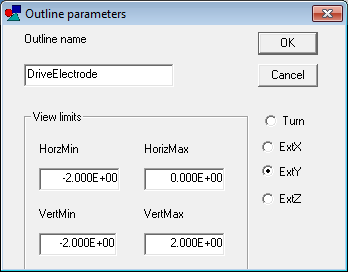
Figure 67: Dialog to start a new outline.
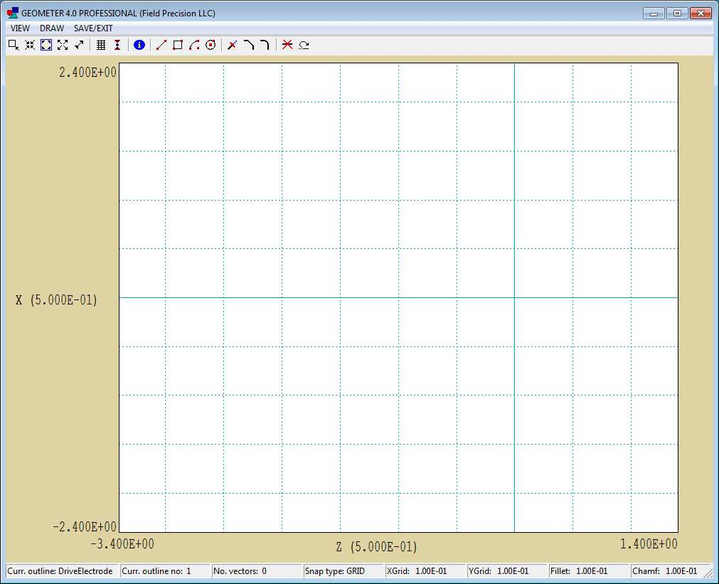
Figure 68: Initial appearance of the Outline Editor.
To make a line, pick Draw/Insert line. Move the cursor to the correct start position and click the left button. Then move to the end position and click the left button again. You can continue making lines by clicking start and end points. When you are finished, click the right button to exit line entry mode. Figure 69 shows the rough outline. We’ll add fillets of radius 0.125 to finish the work. Click Draw/Fillet/chamfer width and enter the value 0.125 in the dialog. Then choose Draw/Fillet. Move the mouse cursor over one of the lines and click the left button to highlight the vector. Then move over the intersecting line and left-click. Geometer completes the fillet, modifying old vectors, adding new ones and reordering the set.
The shape is now complete. Click Save/Exit, choose Save outline and exit. There is now one outline available to define parts in Geometer. Currently, the outline exists only in the program memory and will be lost unless you add it to a part in the MetaMesh script. It’s a good idea to save the outline as a file that you can import into other Geometer sessions. In the main Outline menu, click Save outline and choose an appropriate name and location. The file is in text format and can be inspected or modified with an editor. Here is the content:
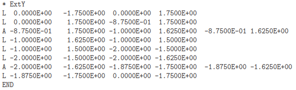
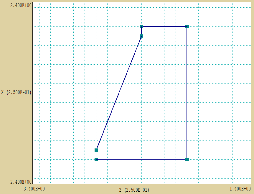
Figure 69: Rough outline before adding fillets.
Exit the Outline Editor. To conclude, we’ll add the final part incorporating the outline. Pick Edit/Add part. In the dialog (Fig. 70), set the Type to Extrusion. Note that the Outline popup menu at the upper-right becomes active. There is only one choice (DriveElectrode). Highlight it and press Enter. The extrusion axis radio buttons beneath change to ExtY. For the model, there is only one fabrication parameter, the Height. Set it to 4.0. Finally, the top of the electrode that we drew at z = 0.00 cm for convenience should coincide with the top boundary of the solution volume (z = 3.00 cm). Accordingly, set Zshift = 3.00 cm. When all values have been set to correspond to those of Fig. 70, click OK. After inspecting plots to check validity, save your work as the MetaMesh input file CapDetector.MIN.
Run MetaMesh and load the file you just created. To start, let’s take a look at it. Choose File/Edit MIN file to display the contents. The top section lists the properties of the foundation mesh, the basic elements to construct the geometry. Geometer has made default choices for the element sizes. We’ll change them so that elements are matched to objects in the assembly. By matched, I mean that the initial boundaries between elements are coincident with the boundaries of many of the objects. Change the foundation-mesh specifications to:
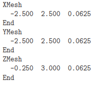
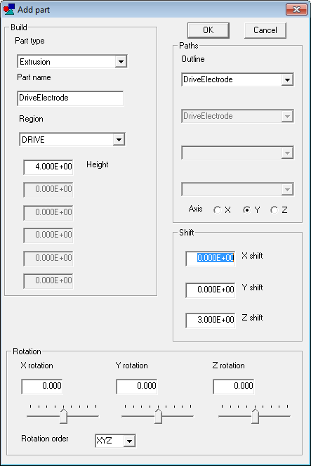
Figure 70: Dialog to define properties of the drive electrode part.
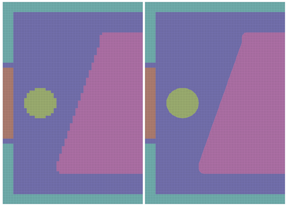
Figure 71: Comparison of meshes without and with region surface fitting.
Save the file and exit the editor. Process the mesh, go to the 2D plot window and choose a plot normal to the y axis. The result looks like the left-hand side of Fig. 6. The metal wall and detector are well represented because of our judicious choice of element sizes. On the other hand, the drive electrode and object have a stair-step shape. To get accurate field interpolations near the surface, we need to instruct MetaMesh to apply conformal fitting (i.e., shift elements near the surface from boxes to generalized hexahedrons with facets that lie on the object boundaries).
Open the MIN file in the text editor again and add Surface commands for the Drive and Object parts as shown in Table 3. The command
Surface Region Air
instructs the code to identify all elements of the part that share facets with the Air region and to change their shape so that they conform to the model surface. Save the file, exit the editor, reload the MIN file and process it. The right-hand side of Fig. 71 shows the improved result. Click File/Save mesh to create CapDetector.MDF.
The task of geometry definition is complete. Modifications to an assembly are generally much easier than the initial creation. You can reload the MIN file into Geometer and quickly change the shape, position and orientation of parts. You could also edit the MIN file directly to move parts around. We’ll make use of this feature to determine the variation of mutual capacitance between the drive and detector electrodes as the position of the object changes. In the next chapter, we’ll discuss the finite-element solution and useful analysis techniques.
Table 3: Drive and Object part specifications in CapDetector.MIN