![]()
17 3D electrostatic application: mutual capacitance
In this chapter, we’ll conclude the application example by calculating the electric field and discussing two useful techniques:
• Determining mutual capacitances in a system with multiple electrodes.
• Setting up HiPhi solutions for automatic operation in the background.
Run HiPhi, click Setup and load CapDetector.MDF. We discussed the Setup dialog in Chap. 14. Its function is to create a HiPhi input script, CapDetector.HIN, to control the field calcula- tion. Here, we’ll concentrate on the contents of the file (Fig. 72). The values at the top are control parameters (mostly defaults). The DUnit command states that the coordinates in the MetaMesh file are given in cm. The remaining commands specify the identity and physical properties of regions. The value of the drive voltage, 1.0 V, is a convenient choice for capaci- tance calculations. Note that there are two entries for the detected Object (Region 5 ), one of which is commented out. To begin, we will calculate the field without the object, equivalent to setting ǫr = 1.0. Click Run in HiPhi and pick CapDetector.HIN to generate the solution file CapDetector.HOU.
Run PhiView and load the solution file. To begin, we’ll make a plot of |E| along x at the position of the object (y = 0.000 cm, z = 0.625 cm) to identify the region of linear field variation. Click Slice plots and choose Slice normal to y. Click Plot control/Plot style and set the style to Element. Click Plot control/Plot quantity and choose |E|. The result is the top plot of Fig. 73. Make sure Analysis/Scan plot quantity is set to Ez. Choose the command Analysis/Line scan. Although you could specify the endpoints of the scan with the mouse, in this case we want to be sure the line is at the horizontal position of the object center. Press the F1 key to type values for the start position: z = 0.625 cm, x = −2.25 cm. Click OK and press F1 again to type the end position: z = 0.625 cm, x = 2.25 cm. PhiView calculates values and displays the graph shown at the bottom of Fig. 73. The region of approximately linear variation covers the range -1.25 cm ≤ x ≤ 1.25 cm.
We will proceed with the calculation of mutual capacitance between the drive and detector electrodes, advancing to a higher level of automatic analysis at each stage. For the discussions, the three electrodes in the solution have been numbered in Fig. 73. We’ll start with single operations that you control in the interactive environment of PhiView, appropriate for one or a few calculations.
The mutual capacitance between electrodes 1 and 2 is given by C12 = Q2/(V1 − V2). The charge induced on the detector is given by the surface integral:
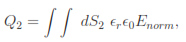 (9)
(9)
where Enorm is the electric field normal to the surface and ǫr is the relative dielectric constant of the medium surrounding the detector. In this case, ǫr = 1.0. The PhiView configuration file phiview dielectric.cfg contains this definition:

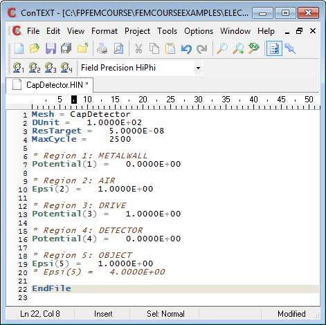
Figure 72: File CapDetector.HIN viewed in ConText.
Here, &Ex is a calculated component of electric field and &Q[2] is the relative dielectric constant. PhiView takes automatic surface integrals over regions by evaluating the quantities of Eq. 9 just outside the facets of the region boundary. The result is the quantity Q2 in coulombs. Because we picked an applied voltage of 1.0 V, the result can also be interpreted directly as the mutual capacitance.
Return to the main PhiView menu and click Analysis/Surface integral to bring up the dialog of Fig. 74. Because PhiView can take integrals over the combined surface of multiple regions, we need to specify which regions are inside the surface and which ones are outside. In this case, the detector is inside and all others are outside as shown. When you click OK, the program prompts you to create a file CapDetector.DAT to record the results. This is a useful feature of numerical work; otherwise, it would be necessary to copy the results from the screen.
To see the results, click File/Close data file and then File/Edit data file. Here is the entry:
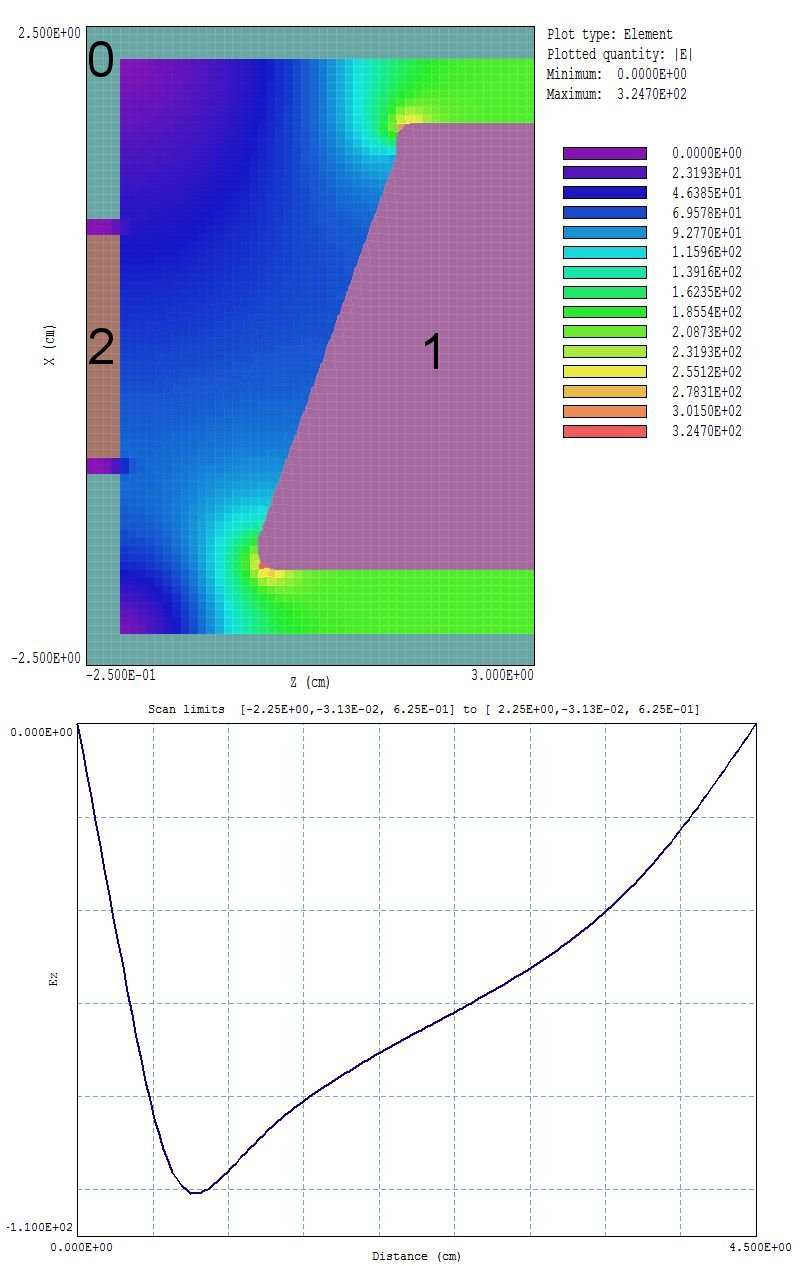
Figure 73: Top: Variation of |E| in the plane y = 0.0 cm. Bottom: Scan of |E| along x at
y = 0.0 cm, z = 0.625 cm.
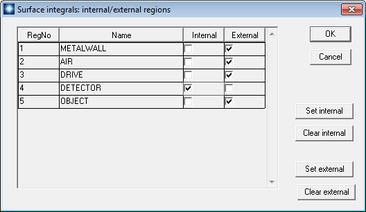
Figure 74: Dialog to control the PhiView surface integral.
---------- Surface Integrals ---------- Region status
RegNo Status Name
===================================0
1 External METALWALL
2 External AIR
3 External DRIVE
4 Internal DETECTOR
5 External OBJECT
Surface area of region set (m2): 8.187500E-04
Charge: -3.015445E-13
The mutual capacitance without the object is 0.30154 pF.
When possible, it’s a good idea to make an analytic estimate to make sure we haven’t made a fundamental error in the numerical setup. The mutual capacitance is approximately
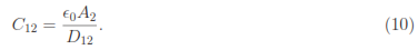
The average distance between the drive and detector is D = 0.015 m. The area of the upper detector surface is A 2 = (0.0175)(0.0325) = 5.7×10 -4 m 2 12 . Substituting in Eq. 10, the estimated capacitance is C 12 = 0.335 pF, close to the code result.
Open the file CapDetector.HIN with an editor and change the object properties to
* Region 5: OBJECT
* Epsi(5) = 1.0000E+00
Epsi(5) = 4.0000E+00
Recalculate the field with HiPhi and find the detector surface integral with PhiView. The result with the object centered at x = 0.0 cm is C12 = 0.3162745 pF. The object raises the mutual capacitance by about 4.9%.
To complete the calculation, we want to find C12 with the object at positions x = -0.50, -0.25, 0.00, 0.25 and 0.50 cm. To analyze each solution, we must load CapDetector.HOU into PhiView and call up the surface integral. Rather than perform the same operations every time, we can define an automatic analysis sequence. In the PhiView main menu, click File operations/Create script. Supply the file prefix CapDetector. The program opens the internal editor with a template of available analysis script operations. Type in information so that the script looks like this:
INPUT CapDetector.HOU
OUTPUT CapDetector.DAT Append
SURFACEINT 4 -1 -2 -3 -5
ENDFILE
Click Save to create the file Surface.SCR and exit the editor. The script specifies the following operations
• Load the HiPhi solution CapDetector.HOU.
• Write information to a data file CapDetector.DAT. The Append directive signals that
PhiView should add data to the file if it exists.
• Perform a surface analysis. The numbers following the command indicate that that Region 4 (the detector) should be inside and all others outside.
To add a value of mutual capacitance to the output file, simply click File operations/Run script in the main menu of PhiView and choose CapDetector.SCR.
A manual run to find C12 for an object position requires the following activities:
1. Edit CapDetector.MIN. To move the object to x = −0.5 cm, change the Shift command in the object section to Shift: -0.500 0.000 0.0625.
2. Run MetaMesh, click File/Load MIN file and choose CapDetector.MIN. Then click Process followed by File/Save mesh.
3. Run HiPhi, click Run/Start run and choose CapDetector.HIN.
4. Run PhiView and start the analysis script CapDetector.SCR.
There are many redundant operations. To start, let’s automate the second, third and fourth activities with a Windows batch file. I’ll assume that you are running the programs from the AMaze program launcher and that the Data folder is set to the working directory. In AMaze, click the Create task button to bring up the dialog of Fig. 75. Fill in the Task prefix as CapDetector. Under Action, click the arrow to activate the popup menu. In contains a list of the 3D programs and common batch operations. Pick MetaMesh. Then, click on the cell under File in and click the Select file button to show a list of MetaMesh input files available in the working directory. Choose CapDetector.MIN. The output file of the activity is always CapDetector.MDF, so we do not need to specify a value. Go to the next Action cell and pick HiPhi. For File in, choose CapDetector.HIN. Set PhiView for the next action with CapDetector.SCR as the input file. When you click OK, AMaze saves the setup as CapDetector.BAT, a standard batch file. Here is the content:
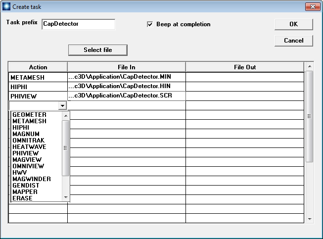
Figure 75: AMaze dialog to create a task.
START /B /WAIT C:fieldp_proamazemetamesh.exe C:...CapDetector
START /B /WAIT C:fieldp_proamazehiphi.exe C:...CapDetector
START /B /WAIT C:fieldp_proamazephiview.exe C:...CapDetector
START /B /WAIT C:fieldp_proamazeNOTIFY.EXE
IF EXIST CapDetector.ACTIVE ERASE CapDetector.ACTIVE
The batch file runs each program in the background with the specified input file, waiting until an operation is complete before moving to the next one. The fourth line calls for an audio signal to mark the end of the sequence. The fifth line deletes a temporary file used to keep track of which tasks are active.
At this stage, we have reduced the work to two user operations for each position of the object:
• Edit the Shift operation in CapDetector.MDF to change the object position along x.
• In AMaze, click the Run task button and choose CapDetector.BAT from the list of available tasks. In response, the mesh is regenerated, the field solution is updated and the surface analysis result is added to the data file CapDetector.DAT.
The end result is a list of C12 values at the different positions.
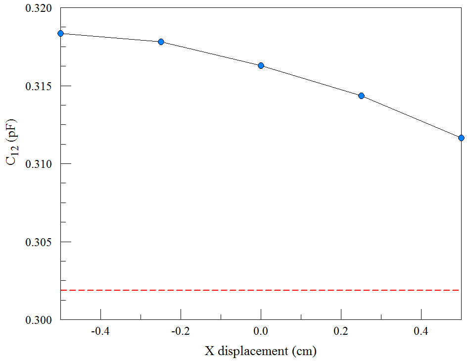
Figure 76: Variation of C12 with the displacement of the dielectric object. The dashed line shows the value with no object.
To conclude, we can eliminate the first task to automate the entire process. Here. we will specify the changing object position within the calling batch file. We need to make two changes. First, the Part section for the object in the MetaMesh input file should be modified to:
PART
Region: Object
Name: Object
Type: Sphere
Fab: 3.75000E-01
Shift: %1 0.00000E+00 6.25000E-01
Surface Region Air
END
Note that the x position in the Shift operation is represented by a variable. The value to be used is given as the first command line parameter when calling MetaMesh. The file CapDetector.BAT should be edited to look like this:
START /B /WAIT C:fieldp_proamazemetamesh.exe C:...CapDetector -0.50
START /B /WAIT C:fieldp_proamazehiphi.exe C:...CapDetector
START /B /WAIT C:fieldp_proamazephiview.exe C:...CapDetector
START /B /WAIT C:fieldp_proamazemetamesh.exe C:...CapDetector -0.25
START /B /WAIT C:fieldp_proamazehiphi.exe C:...CapDetector
START /B /WAIT C:fieldp_proamazephiview.exe C:...CapDetector
...
START /B /WAIT C:fieldp_proamazemetamesh.exe C:...CapDetector 0.50
START /B /WAIT C:fieldp_proamazehiphi.exe C:...CapDetector
START /B /WAIT C:fieldp_proamazephiview.exe C:...CapDetector
START /B /WAIT C:fieldp_proamazeNOTIFY.EXE
IF EXIST CapDetector.ACTIVE ERASE CapDetector.ACTIVE
The task generates the entire data set. Figure 76 shows a plot of the results. The dashed line is the mutual capacitance with no object. The relative variation of C12 with position of the object is about ±1.1%. The conclusions are that the application would require a sensitive detector and that small variations in the size or properties of the dielectric object could overwhelm the measurement.
An alternate way to find mutual capacitance is the energy method described in the HiPhi manual. In this case, it is necessary to make three solutions for each configuration with different combinations of electrode voltages. The capacitance values C12, C10 and C20 are determined by comparing values of the total field energy. The procedure requires 15 solutions – here, the automation features of HiPhi provide a significant benefit. In the calculations, the electrode voltages as well as the object position are set by command line parameters.