![]()
18 3D magnetic fields: defining coil currents
In this chapter, we’ll start the final topic in this book: 3D magnetic field solutions. The previous chapters on electrostatics covered many common techniques for 3D solutions, particularly mesh generation. Here, we’ll focus on the differences between Magnum and HiPhi calculations that arise from the unique characteristics of magnetic fields:
• The vector driving terms for magnetic solutions require more intensive data input.
• Two completely different solution techniques apply in magnetic solutions, depending on whether ferromagnetic materials are present.
• Magnetic materials have more complex properties.
The phrase driving terms refers to the information we must supply to a finite-element pro- gram to create fields. For example, the drivers of electrostatic solutions are differences in the electrostatic potential between electrodes and space-charge. In other words, we apply a fixed potential to the nodes of a region of the solution volume or define space-charge density ρ over elements of a region. In both cases, the specified quantities are scalar. For either drive type, we must employ the finite-element technique to determine the self-consistent charge density on electrode surfaces.
There are two possible drives in magnetic-field solutions:
• Currents in coils.
• Material currents in permanent magnets.
Coil currents constitute a unique challenge in 3D solutions. To review, we saw in Chap. 7 that it was easy to define currents in 2D solutions. In cylindrical geometries, current flowed only in θ and in planar solutions the current flow was along z. In other words, current was a scalar quantity assigned to regions that represented the cross sections of coils. In 3D solutions, the drive current is a vector quantity that can flow anywhere. If you think about devices like electric motors, it’s clear that drive coils may be highly complex assemblies. The implication is that the definition of drive coils is a significant task in 3D solutions, on a par with mesh generation. In consequence, the Magnum package contains a utility MagWinder specifically for coil windings.
Next, consider options for magnetic solution procedures. Suppose we have a set of drive coils in a system with no ferromagnetic materials. (In other words, all objects in the solution space have relative magnetic permeability µ0 = 1.0.) In this case, there are no unknown currents. The field at any point can be determined by a Biot-Savart integral14 over the drive current elements. It is not necessary to build a conformal mesh of regions or even to apply the finite– element method. On the other hand, a mesh and a finite-element solution are essential when the solution space contains permanent magnets or magnetic materials (µr = 1.0). Here, material currents that are not known a priori have a significant effect on the fields. The implication is that a 3D magnetic field program should be capable of two different types of calculations.
14Section 9.1 of the book Finite-element Methods for Electromagnetics reviews the Biot-Savart law.
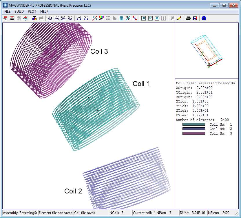
Figure 77: Demonstration coil assembly displayed in the MagWinder working environment.
Finally, let’s address the nature of materials. In electrostatic solutions, dielectrics have a moderate influence on the total fields and preserve their properties over the practical range of field intensity. An isotropic dielectric can be characterized by a single value of relative dielectric constant ǫr (usually in the range < 100) that changes little all the way to breakdown. In contrast, values of the relative magnetic permeability for iron and other ferromagnetic materials may exceed 10,000 at low field levels. In other words, these materials sustain large surface currents and have a strong effect on the total field. The challenge follows from the fact that the materials may become saturated at field levels encountered in practical systems. Here, the value of µr depends on the local level of magnetic flux density. A magnetic field program must be capable of handling nonlinear solutions.
In the coming articles, we’ll work through two application examples. The first demonstrates the free-space solution type (i.e, no magnetic materials). We’ll investigate the stray fields gen- erated by a heater coil at the emission surface of a thermionic cathode. The second application, the holding force of a latching solenoid, demonstrates a full finite-element solution. It involves drive coils, permanent magnets and high-permeability steel. Both applications require work with MagWinder. In the remainder of this chapter, we’ll get familiar with the program.
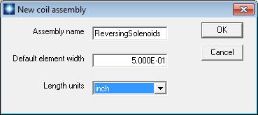
Figure 78: Dialog to start a new drive coil assembly.
Figure 77 shows the coil assembly we will construct, part of a transport system for a high- current electron beam. The full assembly is an array of solenoid lenses with alternating polarity to focus the beam through a 90o bend. The bend is centered at the origin of the y-z plane at x = 0.0”. The bend radius from the origin to the solenoid centers is 20.0”. We will build three of the coils with total amp-turns I = 20 kA, -20 kA and -20 kA. We’ll start with the middle coil. Click the MagWinder button in the AMaze program launcher15. Click File/New coil assembly. In the dialog of Fig. 78, supply the name ReversingSolenoids and set the length units to inches.
Some explanation is required to understand the quantity Default element width. For the Biot-Savart integral, wires are divided into a large number of short elements. In the present setup, we will divide each current loop in the solenoid into 20 azimuthal pieces. Although the elements are plotted as thin wire segments, they are not treated that way in Magnum. Infinitely-thin wires would give rise to discontinuous, diverging values for the applied field. Instead, each element is treated as a cylinder of uniform current density with a diameter equal to its length. Therefore, the wires of Fig. 77 act more like current density layers than a set of discrete filaments.
Next we need to add coils to the assembly. We’ll start with the middle coil. The central field points along z. The center is displaced 20.0” along y. Click Build/New coil to display the dialog of Fig. 79. Fill out the values as shown. Then click OK. A coil is data structure that may contain one or more physical parts. In order to see a plot, we need to add a part. Click Build/Add part to open the dialog of Fig. 80. MagWinder includes several predefined models – the solenoid is one of the most useful. Note that the active fields and labels change when you choose the model. The values shown in Fig. 80 designate that the solenoid has inner radius 2.5”, outer radius 3.0” and a length 3.0”. The radial thickness is represented by two layers. There are 20 sets of circular coils along the axial direction for a total of 40. Each circle is divided into 20 parts. Therefore, MagWinder will create 800 current elements to represent the solenoid. Note that the positions and rotations of parts are taken relative to the encompassing coil. We’ll leave the quantities at the bottom of the dialog at their default values. For the other solenoids, we will apply shifts and rotations to the encompassing coils. Click OK when you are finished entering values. Figure 81 shows the MagWinder display of the first coil16.
15The MagWinder button becomes active when Magnum is installed.
16The three coils of the assembly each contain one part (a solenoid). An example of a coil with multiple parts is a solenoid with wire leads.
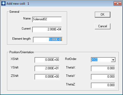
Figure 79: Dialog to add a coil to the assembly.
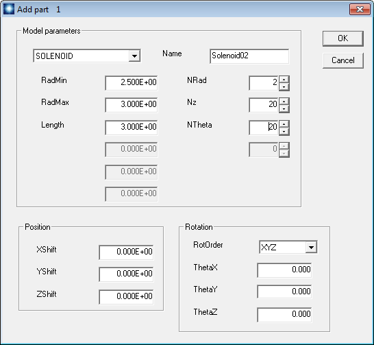
Figure 80: Dialog to add a solenoid part.
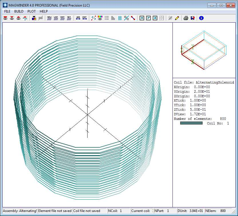
Figure 81: MagWinder display with one coil added.
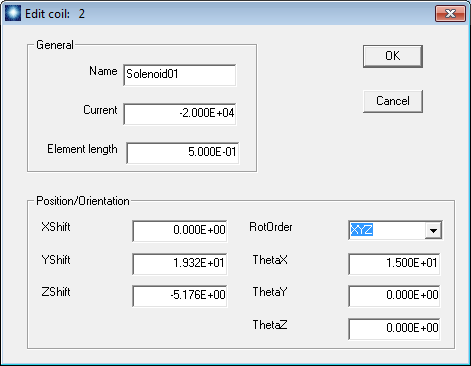
Figure 82: Dialog to add a second coil to the assembly.
The second coil is identical to first except that it is rotated -15o about the x axis at the origin of the y-z plane and has a current of -20 kA. Click File/New coil assembly. Fill in the dialog with the values shown in Fig. 82. For reference, the displacement in z is 20.0 sin(−15o) and in y is 20.0 cos(−15o). A rotation of +15o about the x axis aligns the solenoid with the beam axis. Rather than redefine the solenoid part in an Add part dialog, we will copy and paste the part from the first coil. Click Build/Set current coil and pick the first coil. Then click Build/Copy part and pick the solenoid. Use Build/Set current coil to return to the second coil and click Build/Paste part. When you click OK, the plot shows both coils. The total number of elements is 1600. Use a similar procedure to create a third coil rotated +15o about the y-zorigin.
Assuming the assembly looks like Fig. 1, we need to save the work. There are two types of output files:
• The coil-definition-file (CDF) is a symbolic representation of the coil geometry. This file may be reloaded and modified.
• The winding file (WND) is a list of current elements, input for Magnum. A WND file can always be regenerated from the CDF file, but the CDF file cannot be inferred from information in the WND file.
Both files are in text format. Click File/Save coil file to make the file ReversingSolenoids.CDF. You can view it with the internal program editor. By now, the conventions of the script formats should be familiar. It it easy to recognize the values you entered via the interactive dialogs. Finally, click File/Save element file to generate ReversingSolenoids.WND. Again, this well- formatted file can be inspected with an editor. Here is an excerpt:
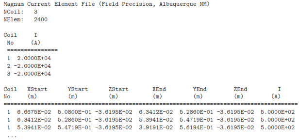
There are 2400 element data lines. Dimensions have been converted to meters for input to Magnum. There are 40 current loops per solenoid, so each loop carries 20000/40 = 500 A.
In the next chapter, we’ll concentrate on the free-space mode of Magnum. We’ll calculate the field for this assembly, and then follow the application example for the cathode heater.