![]()
3 First 2D electrostatic solution
In this chapter, well run through the steps of a solution and analysis of a 2D electrostatic problem without going into detail. The goal is a quick demo of the capabilities of EStat. Subsequent articles will cover details of program techniques.
A notable feature of our programs is dual input - there are two options for supplying geometric and material data for solutions:
• Interactive: the standard method for modern finite-element programs where you fill in items in dialogs. This option is useful for new users and for a quick setup of a new system.
• Text: the classic method using input scripts. This option allows experienced users to make changes to setups easily and facilitates automatic program operation under the control of external programs or batch files. Scripts also provide a permanent archive of setups.
In this demo calculation, we will check out prepared input scripts before running them using the built-in text editors of Mesh and EStat. For serious work, its essential to have a good text editor. This blog article describes how to obtain the ConText editor and how to add syntax color coding for our programs:
http://fieldp.com/myblog/2014/using-the-context-text-editor-update/
Before starting, we’ll need to make some provisions for data organization. A little effort in the beginning circumvents headaches later. Run FP File Organizer or your own file manager. Navigate to a location where you would like to create a general directory (folder) for your finite-element calculations and create the directory Simulations (I will use C:Simulations). Create the sub-directories Electrostatics and ElectrostaticsPractice. In the right-hand window, navigate to C:fieldp basictricompExamplesEStatExamples. We will copy an example for our work. Highlight the files with name ElectronDiode and copy them to the Practice directory. Figure 7 shows the resulting setup in FP File Organizer.
Click on the desktop shortcut to run the TriComp program launcher tc.exe (Fig. 8). The Mesh and EStat buttons should be active as shown. If not, click the Program folder button and navigate to C:fieldp basictricomp. Click the Data folder button and navigate to c:SimulationsElectrostaticPractice. Subsequently, all input/output operations will target this folder.
There are three steps in a finite-element solution:
• Define the geometry of the solution space and divide objects into small volumes (ele- ments). The process is called mesh generation.
• Create and solve a large set of linear equations to approximate the governing partial differential equation (such as the Poisson equation for electrostatics). The goal is to determine the electrostatic potential on points of the mesh (nodes).
• Analyze the results - use the potential values to find physical quantities of interest (e.g., electric field, field energy, capacitance,....).
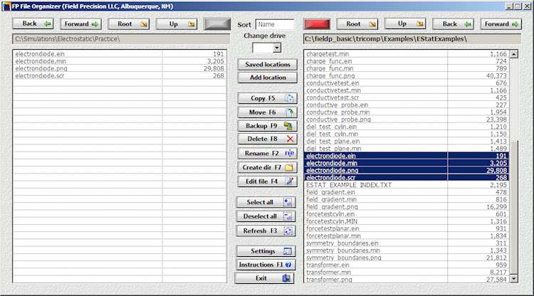
Figure 7: Set up a data directory and copy the examples.
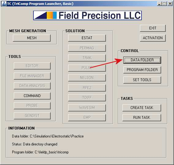
Figure 8: The TriComp program launcher.
The first function is performed by the Mesh program (mesh.exe) and the second and third functions are performed by the EStat program (estat.exe). Meshing is performed by a separate program because the same mesh may be used for different types of solutions. Output from Mesh is compatible with PerMag (magnetic fields), TDiff (thermal transport) and other solution programs of the TriComp series. In other words, what we learn about Mesh for electrostatics is also useful for the magnetic solutions we will discuss later.
Click the Mesh button to open the program. Initially, the screen is blank. Choose File/Edit file from the menu at the top. The selection dialog shows the four files in the data folder. Pick ElectronDiode.MIN, where MIN designates Mesh INput. The internal editor shows the file contents (Fig. 9), a set of organized numbers. For now, note that there are Region sections that represent the different physical objects in the solution space. Each region section contains a set of line or arc vectors that gives the region shape. The numbers are the coordinates of the vectors. There are two ways to create or to modify the content of MIN files:
• Use the Mesh Drawing Editor, an interactive 2D CAD program.
• Use a text editor to change numbers directly.
We will discuss both options in following articles. For now, exit the editor with no changes.
Choose File/Load script(MIN) in the menu or use the Open-file tool on the left hand side of the toolbar to load the contents of the file ElectronDiode.MIN. Then pick Process or click the tool with the green square. In response, Mesh analyzes the desired element sizes and the region vectors to create a set of small elements. To view the result, choose Plot/Repair from the menu or click the Plot/repair tool to show the display of Fig. 10. The solution volume has been divided into the regions listed in the script to represent physical objects (electrodes and dielectrics). The cross section has been divided into triangular areas. Note that the calculation represents a cylindrical system, a figure of revolution about the bottom boundary (r = 0.0). When first viewing a z-r plot, many users ask wheres the bottom? The answer is that there is no bottom. Negative values of the radius r are undefined. On the other hand, a plot in a Cartesian slice plane like y = 0.0 would have both upper and lower components. In cylindrical solutions, elements are tori with triangular cross-sections that extend over the full range of azimuth (θ = 0o to 360o).
Lets take a closer look at the solution. Choose View/Zoom window and specify the corners of a box by moving and left-clicking the mouse. Figure 11 shows a magnified view for a better look at the element cross-sections. The inset at lower-right shows the view limits. Note that the triangles were flexed for a good match to region boundaries. The fitting allows high-accuracy calculations of surface fields. A mesh with element shapes customized to the geometry is called a conformal mesh. To conclude work with Mesh, return to the main menu and choose File/Save mesh (MOU). Refresh the display in FP File Organizer (press F3). Two new files have been added to the folder:
• ElectronDiode.MLS: a text listing file of diagnostic information that may be useful if there is a problem.
• ElectronDiode.MOU: the main output file specifying element identity (region association) and coordinates of nodes (boundaries between elements). This file may be ported to any of the TriComp solution programs. The file is in text format, so you can inspect it with an editor.
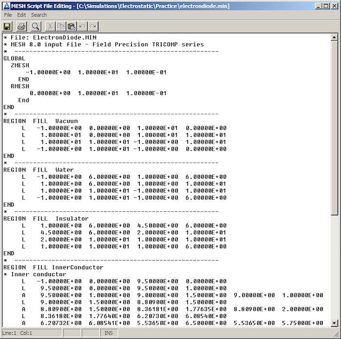
Figure 9: Internal Mesh editor display.
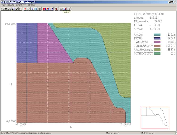
Figure 10: View of the full mesh.
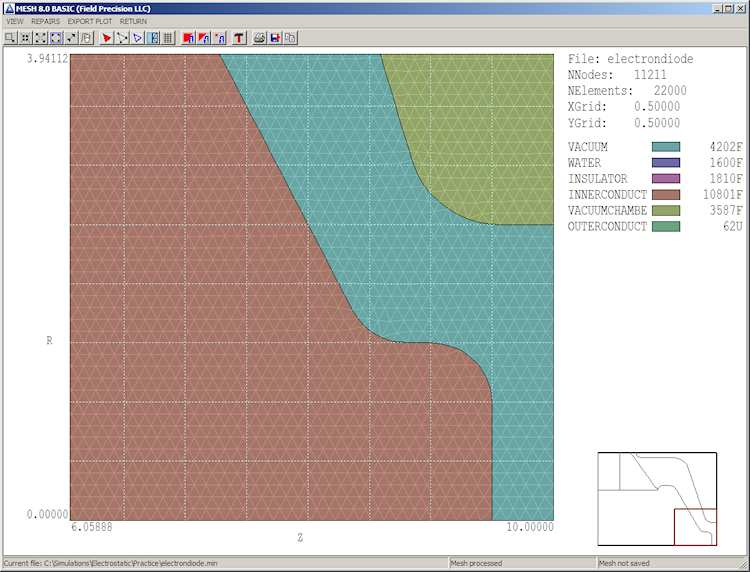
Figure 11: Detailed view of a mesh section.
Next, run EStat from the program launcher. Choose File/Edit script (EIN) and pick the file ElectronDiode.EIN. The editor shows the content
* File ElectronDiode.EIN DUnit = 39.37
Geometry = Cylin
Epsi(1) = 1.0
Epsi(2) = 81.0
Epsi(3) = 2.7
Potential(4) = -500.0E3
Potential(5) = 0.0E3
Potential(6) = 0.0E3
ENDFILE
The two general commands at the top specify that the dimensions from the Mesh file should be interpreted in inches and that the system has cylindrical symmetry. The other commands set the physical properties of regions of the solution volume. The first three regions are dielectrics (vacuum, purified water and cast epoxy) and the other regions are fixed-potential electrodes. Again, there are two options for creating EStat input scripts - supplying values in an interactive dialog or direct input with a text editor.
The tools labeled 1, 2 and 3 invoke the three main functions of EStat:
• Create the input script.
• Perform the finite-element solution.
• Analyze the results.
Step 1 has already been performed, so click the tool marked 2 and pick ElectronDiode.EIN. EStat reads the geometry data in ElectronDiode.MOU, generates the set of finite-element coupled linear equations and solves them, all within a second. FP File Organizer shows that two new files have been created: ElectronDiode.ELS (a diagnostic text listing file) and ElectronDiode.EOU (the main solution file containing potential values at nodes). Click the 3 tool in EStat and pick ElectronDiode.EOU. The program shifts to the Analysis menu and displays the default equipotential-line plot of Fig. 12. This type of plot is useful for experienced users because it shows complete information. Section 7.5 of the companion text Finite-element Methods for Electromagnetics describes how to interpret equipotential plots.
There are many capabilities of the Analysis menu that you can explore. Lets check out two of them. A plot of the magnitude of the electric field |E| is useful to pinpoint areas where breakdowns may occur in high-voltage systems. To create the plot, press Plots/Plot settings/Plot type in the menu and choose Element. Then press Plots/Plot settings/Plot quantity and pick |E|. The resulting plot (Fig. 13) shows that the peak field in the electron emission region is about 442 kV/cm and that the maximum field on the insulator vacuum surface is about 40 kV/cm. A second activity is to find the capacitance of the system downstream from the insulator. We can determine this quantity from the volume integral of electrostatic field energy density in the vacuum region. Press Analysis/Volume integral. EStat offers to open a data record file with the default name ElectronDiode.DAT. Global information will appear on the screen, but we need to check the file for a detailed breakdown by regions.
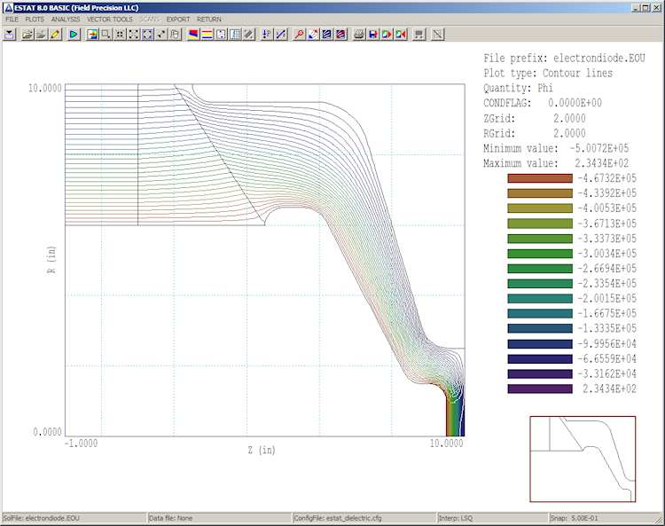
Figure 12: Equipotential line plot of the electrostatic solution.
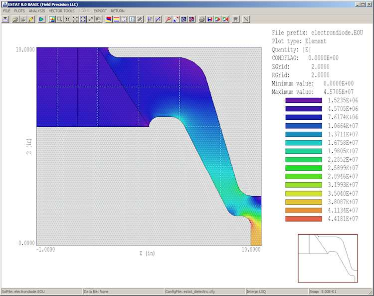
Figure 13: Variation of electric field magnitude in the solution volume.
Press File/Close data record and then File/Edit files. Open ElectronDiode.DAT. Here is the information of interest:
Quantity: Energy
Global integral: 6.358995E+01
RegNo Integral
==========================
1 5.534785E+00
2 5.602793E+01
3 2.027232E+00
4 4.472539E-29
The capacitance of the vacuum volume (Region 1) may be determined from the equation Ue =
CV 2/2 as (2)(5.5347/(5.0 × 105)2 = 44.3 pF.
We have completed the first electrostatic solution. An inspection of the final state of the data folder shows two features of Field Precision programs:
• The compact input files ElectronDiode.MIN and ElectronDiode.EIN contain complete information to reconstruct the solution.
• All the data that we generated has been recorded in accessible files. For example, if you archive the file ElectronDiode.EOU, you can always return for additional analyses.
The purpose of this example was to give an overview of the program features. In following chapters, we shall create solutions from scratch, learning about meshing and analysis techniques.