EI π
2
f =
i +
i =
(70)
i
(4
1) ,
1,2,L,5
2
m 32 L
where E is the modulus of elasticity of Joung (
11
2
≅ 10 N / m ),
4
I = l /12 is the moment of
inertia of the section respect to the deflection axis and
2
m ≅ 7876 l Kg/ m is the mass per unit
length of the link, are:
An Innovative Method for Robots Modeling and Simulation
195
f = 6.31, 20.4, 42.7, 73.0, 111.3 Hz .
(71)
C
F
α
d
d
δ
Cc
β
Fig. 14. Schematic representation of a single-link flexible arm.
The frequencies obtained with the proposed method, dividing the link into five and ten
flexible sublinks, respectively result:
f = 6.31, 20.4, 41.9, 65.6, 90.8Hz
(72)
f = 6.31, 20.4, 42.6, 72.77, 110.5Hz .
(73)
Stressing the link with C = − Nm C = Nm F = N , if β = 0 , the theoretic values of
c
1
, d 1
, d 0
α and δ are:
2
L
L
α =
C =
° δ =
C =
cm .
(74)
d
1.375 ,
d
2.40
EI
2 EI
It is worth noting that these values and the ones obtained using the proposed method are
coincident 1
ν
∀ ≥ (Celentano, 2007).
Applying to the link C = − Nm C = Nm F = N , if β = 0 , the theoretic values of
c
2
, d 0
, d 1
α and δ result:
2
3
L
L
α =
F =
° δ =
F =
cm .
(75)
d
1.375 , 3.20
2 EI
3
d
EI
The first value (the orientation angle of payload due to the arm deflection) and the ones
computed with the proposed method ν
∀ ≥ 1 are coincident, while the second value (the
motion of the payload due to the arm deflection) obtained using the proposed method has a
relative error of (Celentano, 2007)
1
⎧
0.01
−
= 1%,
if 5
ν =
ε = −
=
δ
⎨
(76)
2
4ν
0.0025
−
= 0.25%, if 10.
ν =
⎩
6. Conclusion
In this chapter an innovative method for robots modeling and simulation, based on an
appropriate mathematical formulation of the relative equations of motion and on a new
196
New Approaches in Automation and Robotics
integration scheme, has been illustrated. The proposed approach does require the
calculation of the inertia matrix and of the gradient of the kinetic energy only. It provides a
new analytical-numerical methodology, that has been shown to be simpler and numerically
more efficient than the classical approaches, requires no a priori specialized knowledge of
the dynamics of mechanical systems and is formulated in order to allow students,
researchers and professionals to easily employ it for the analysis of manipulators with the
complex-shaped links commonly used in industry.
In the case of planar robots with revolute joints, theorems have been stated and proved that
offer a particularly simple and efficient method of computation for both the inertia matrix
and the gradient of the kinetic energy. Then a comparison has been made in terms of
efficiency between the proposed method and the Articulated-Body one.
Moreover, for spatial robots with generic shape links and connected, for the sake of brevity,
with spherical joints, several theorems have been formulated and demonstrated in a simple
manner and some algorithms that allow efficiently computing, analytically the inertia
matrix, analytically or numerically the gradient of the kinetic and of the gravitational energy
have been provided. Furthermore, also in this case a comparison of the proposed method in
terms of efficiency with the Articulated-Body one has been reported.
Finally, a methodology for flexible robots modeling, that allow obtaining, quite simply,
accurate and efficient, from a computational point of view, finite-dimensional models, has
been provided. This method is illustrated with a very significant example.
7. References
Celentano, L. (2007). An Innovative and Efficient Method for Flexible Robots Modeling and
Simulation. Internal Report, Dipartimento di Informatica e Sistemistica, Università
degli Studi di Napoli Federico II, Napoli, Italy, October 2007
Celentano, L. and Iervolino, R. (2007). A Novel Approach for Spatial Robots Modeling and
Simulation. MMAR07, 13th IEEE International Conference on Methods and Models in
Automation and Robotics, pp. 1005-1010, Szczecin, Poland, 27-30 August 2007
Celentano, L. and Iervolino, R. (2006). A New Method for Robot Modeling and Simulation.
ASME Journal of Dynamic Systems, Measurement and Control, Vol. 128, December
2006, pp. 811-819
Celentano, L. (2006). Modellistica e Controllo dei Sistemi Meccanici Rigidi e Flessibili. PhD
Thesis, Dipartimento di Informatica e Sistemistica, Università degli Studi di Napoli
Federico II, Napoli, Italy, November 2006
De Wit, C.C., Siciliano, B. and Bastin, G. (1997). Theory of Robot Control, (2nd Ed.) Springer-
Verlag, London, UK
Featherstone, R. and Orin, D.E. (2000). Robot Dynamics: Equations and Algorithms.
Proceedings of the 2000 IEEE International Conference on Robotics and Automation, pp.
826-834
Featherstone, R. (1987). Robot Dynamics Algorithms, Kluwer Academic Publishers, Boston/
Dordrecht/ Lancaster
Khalil, W. and Dombre, E. (2002). Modelling, Identification and Control of Robots, Hermes
Penton Science, London, UK
Sciavicco, L. and Siciliano, B. (2000). Modeling and Control of Robot Manipulators, (2nd Ed.)
Springer-Verlag, London, UK
11
Models for Simulation and Control of
Underwater Vehicles
Jorge Silva1 and João Sousa2
1Engineering Institute of Porto
2University of Porto
Portugal
1.Introduction
Nowadays, the computational power of the average personal computer provides to a vast
audience the possibility of simulating complex models of reality within reasonable time
frames. This chapter presents a review of modelling techniques for underwater vehicles
with fixed geometry, giving emphasis on their application to real-time or faster than real-
time simulation.
In the last decade there was a strong movement towards the development of Autonomous
Underwater Vehicles (AUV) and Remotely Operated Vehicles (ROV). These two classes of
underwater vehicles are intended to provide researchers with simple, long-range, low-cost,
rapid response capability to collect pertinent environmental data. There are numerous
applications for AUV and ROV, including underwater structure inspection, oceanographic
surveys, operations in hazardous environments, and military applications. In order to fulfil
these objectives, the vehicles must be provided with a set of controllers assuring the desired
type of autonomous operation and offering some aid to the operator, for vehicles which can
be teleoperated.
The design and tuning of controllers requires, on most methodologies, a mathematical
model of the system to be controlled. Control of underwater vehicles is no exception to this
rule. The most common model in control theory is the classic system of differential
equations, where x and u are denominated respectively state vector and input vector:
&x = f (x,u) (1)
In this framework, the most realistic models of underwater vehicles require f(x,u) to be a
nonlinear function. However, as we will see, under certain assumptions, the linearization of
f(x,u) may still result in an acceptable model of the system, with the added advantage of the
analytic simplicity.
On the other hand, simulation, or more specifically, numerical simulation, does not require
a model with the conceptual simplicity of Eq.(1). In this case, we are not concerned with an
analytic proof of the system’s properties. The main objective is to compute the evolution of a
set of state variables, given the system’s inputs.
The hydrodynamic effects of underwater motion of a rigid body are well described by the
Navier-Stokes equations. However, these equations form a system of nonlinear partial
198
New Approaches in Automation and Robotics
differential equations whose solution is very hard to compute for general problems.
Computational fluid dynamics deal with the subject of solving these equations. However,
even with today's computer technology and software packages, the time to obtain the
solution on average computer, even for simple scenarios, is still far from real-time. This kind
of simulation may return very accurate results, but the computation times are not acceptable
if simulation of long term operation is desired. These models are just too complex for control
design and approximations are used for this purpose.
If near, or faster than, real-time simulations are desired, acceptable results can be obtained
by simulating the model employed in the control design. Real-time response is most useful
when teleoperation simulation is desired. In this case, as in car or flight simulators, the user
interacts with the underwater vehicle simulator by setting references or direct actuator
commands on a graphical user interface.
Usually we are interested in checking the performance of the vehicle’s controllers in a set of
operation scenarios. This is done because the control design may involve certain
simplifications or heuristic methods which make it difficult to analytically characterize
certain parameters of the system’s response, such as settling time or peak values
(overshoots) during transient phases of operation. Simulation is an important tool for
controller tuning and for exposing certain limit situations (e.g., actuator saturation) that may
be hard to describe analytically on the model employed for control design.
The typical design cycle involves the test of different control laws and navigation schemes.
In most cases, the control system must be replicated in a simulation environment, usually on
a different language. Even when that is done correctly, it is difficult to keep consistency
between that implementation and the final control system, which may be subject to updates
from other sources. It is possible, as described in (Silva et al. 2007), to have a single
implementation of the control software to function unmodified in both real-life and
simulated environments. Instead of writing separate code first for a prototyping
environment and then for the final version, this approach allows the employment of the
stable/final software in the overall design cycle. Therefore, the simulation may be seen also
as a debugging tool of the overall software design process. Underwater vehicle’s mission
management, with special regards to autonomous operation, may involve complex logic,
besides the continuous control laws. It is of the major importance to test the implementation
of that logic, namely switching between manoeuvres, manoeuvre coordination, event
detection, etc. Since real-life missions may last for some hours, it is quite useful to simulate
these missions in compressed simulated time.
The literature from naval architecture proposes several models for underwater vehicles
following the structure of Eq.(1). The main difference between these models is the way how
the hydrodynamic phenomena associated with underwater rigid body motion is modelled.
The model described in (Healey & Lienard, 1993) is used in many works. These authors
refine a model that can be traced back to 1967 (Gertler & Hagen, 1967) in order to describe a
box shaped AUV. Most recent works use the framework presented on (Fossen, 1994) which,
while less descriptive than the one of (Healey & Lienard, 1993), is more amenable to direct
application of tools from nonlinear control. Recent research on underwater vehicle’s motion
equations can still be found, for instance on (Nahon, 2006).
However, in general, the literature only provides the general equations of the models. These
models are parametrized by tens (sometimes over one hundred) of coefficients. Some of
these coefficients can be easily computed based on direct physical measurements (mass,
Models for Simulation and Control of Underwater Vehicles
199
length, etc.). However, the computation of the coefficients related to hydrodynamic effects is
not a straightforward task. When considering new designs, the accurate estimation of some
of the coefficients, mainly those associated with hydrodynamic phenomena, usually
requires hydrodynamics tests. Although ingenious techniques can be used, see for instance
(von Ellenrieder, 2006), these tests are usually expensive or involve an apparatus which is
not justifiable for every institution.
Certain software packages can be used to obtain more accurate parameters. For instance,
(Irwin & Chavet, 2007) present a study comparing results obtained with Computational
Fluid Dynamics with those of classical heuristic formulas. However, software packages for
this purpose are usually expensive, or of limited accessibility.
The simplest alternative approaches rely on empirical formulas, or on adapting the
coefficients from well-proved models from similar vehicles. In fact, empirical results show
that, for vehicles of the same shape, the hydrodynamic effects can be normalized as a
function of scale and vehicle’s operating speed. For instance, the work of (Healey & Lienard,
1993) presents the complete set of numeric parameters for the model proposed by the
authors on that work. However, the later method is suitable only for vehicles with similar
shape to those whose models are known and the former requires the vehicle being modelled
to follow closely the assumptions of the empirical formulas.
In what follows, we review a standard nonlinear model derived from (Fossen, 1994),
describe further aspects of the hydrodynamic phenomena, and explain how the symmetries
of the vehicle can be explored in order to reduce the number of considered coefficients.
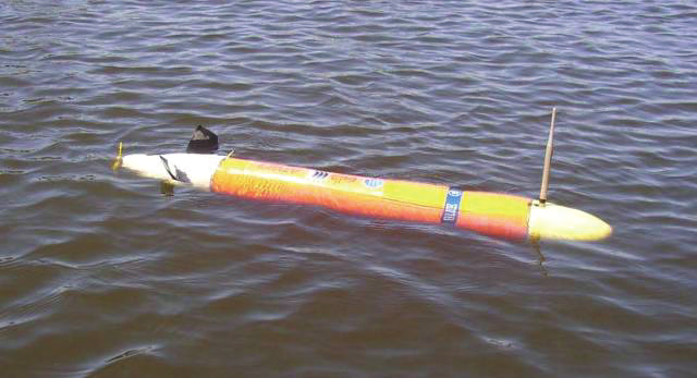
The final conclusions are drawn based on our experiments with the Light Autonomous
Underwater Vehicle (LAUV) designed and built at University of Porto (see Fig. 1). LAUV is
a torpedo shaped vehicle, with a length of 1.1 meters, a diameter of 15 cm and a mass of
approximately 18 kg. The actuator system is composed of one propeller and 3 or 4 control
fins (depending on the vehicle version), all electrically driven. We compare trajectories
logged during the operation of the LAUV with trajectories obtained by simulation of the
vehicle’s mathematical model.
Fig. 1. Light Autonomous Underwater Vehicle (LAUV) designed and built at University of
Porto.
2. Underwater vehicle dynamics
When discussing underwater vehicle dynamics we typically consider two coordinate
frames: the Earth-Fixed Frame and the Body-Fixed Frame.
200
New Approaches in Automation and Robotics
The Earth-Fixed Frame defines a coordinate system with origin fixed to an arbitrary point
on the surface of the Earth and following the north-east-down convention: x points due
North, y points due East, and z points toward the center of the Earth. For marine
applications, this frame is considered the inertial frame.
In the Body-Fixed Reference Frame the origin and axes of the coordinate system are fixed
with respect to the (nominal) geometry of the vehicle. The orientation of the axes is as
shown on Fig. 2: if the underwater vehicle has a plane of symmetry (and we will assume
here that they all do) then xB and zB lie in that plane of symmetry. xB is chosen to point forward and zB is chosen to point downward. Usually the body axes coincide with the
principal axes of inertia of the vehicle. Fig. 2 shows one possibility. The origin of the body-
fixed frame is frequently chosen to coincide with the center of gravity. This is a natural
choice given the equations of rigid body motion. However, in many situations, most
remarkably during prototyping, the center of mass may be changing relatively to the
vehicle’s geometry. That makes necessary to recalculate the moments due some of the forces
involved on vehicle’s motion (e.g., forces due to the actuators). Therefore, in those cases, a
more useful choice would be a point relative to the vehicle’s shape such as the center of
pressure (described later) or simply the geometrical center.
xB
yB
zB
Fig. 2. Body-Fixed Reference Frame.
The minimum set of variables that completely describe the vehicle’s position, orientation,
and linear and angular velocities is called vehicle state. The most commonly chosen state
variables are the inertial position and orientation of the vehicle, and its body-fixed linear
and angular velocities. The orientation of the vehicle with respect to inertial space can be
described by the Euler angles. These angles are termed yaw angle (ψ), pitch angle (θ) and
roll angle (φ). This implies three different rotations will be needed (one for each axis). The
order in which these rotations are carried out is not arbitrary. The standard coordinate
systems and rotations (Lewis, 1989), are as defined in Fig. 3. In what follows, the notation
from the Society of Naval Architects and Marine Engineers (SNAME) is used (Lewis, 1989).
The motions in the body-fixed frame are described by 6 velocity components u, v, w, p, q
and r. Let us define the following vectors:
ν = [u v w]T (1)
1
ν = [p q r]T (2)
2
ν = [ T
ν
ν
(3)
1
]T
T
2
The body fixed linear velocities u, v and w are termed, respectively, surge, sway and heave.
We adopt the following convention: when considering slow varying ocean currents, these
velocities are relative to a coordinate frame moving with the ocean current.


Models for Simulation and Control of Underwater Vehicles
201
The vehicle’s position and orientation in the inertial frame are defined by the following
vectors:
η = [x y z]T (4)
1
η = φ θ ψ
2
[
]T
(6)
η = [ T
η
η
1
2 ]T
T
(5)
x3
φ&
ψ
θ&
θ
x2
y1
φ
y3
ψ
φ
θ
ψ
z
&
2
z1
Fig. 3. Euler angles definition: yaw, pitch and roll.
The twelve basic states of an underwater vehicle may therefore be written as (again, this is
just one possible choice, but it is the standard one):
Name Description Unit
u
Linear velocity along body-fixed x-axis (surge)
m/s
v
Linear velocity along body-fixed y-axis (sway)
m/s
w
Linear velocity along body-fixed z-axis (heave)
m/s
p
Angular velocity about body-fixed x-axis
rad/s
q
Angular velocity about body-fixed y-axis
rad/s
r
Angular velocity about body-fixed z-axis
rad/s
ψ
Heading angle with respect to the reference axes
rad
θ
Pitch angle with respect to the reference axes
rad
φ
Roll angle with respect to the reference axes
rad
x
Position with respect to the reference axes (North)
m
y
Position with respect to the reference axes (East)
m
z
Position with respect to the reference axes (Down)
m
Table 1. Vehicle States
2.1 Dynamic equations
The evolution of η is defined by the following kinematic equation:
η& = (
J η ν (6)
2 )
202
New Approaches in Automation and Robotics
This equation defines the relationship between the velocities on both reference frames, with
the term J(η