The most important single linear integrated circuit is the operational amplifier. Operational
amplifiers (op-amp) are available as inexpensive circuit modules, and they are capable of
performing a wide variety of linear and nonlinear signal processing functions (Stanley,
1994).
In simple cases, where the interest is the configuration gain, the ideal op-amp in linear
circuits, is used. However, the frequency response and transient response of operational
amplifiers using a dynamic model can be obtained.
The bond graph methodology is a way to get an op-amp model with important parameters
to know the performance. A bond graph is an abstract representation of a system where a
collection of components interact with each other through energy ports and are place in the
system where energy is exchanged (Karnopp & Rosenberg, 1975).
Bond graph modelling is largely employed nowadays, and new techniques for structural
analysis, model reduction as well as a certain number of software packages using bond
graph have been developed.
In (Gawthrop & Lorcan, 1996) an ideal operational amplifier model using the bond graph
technique has been given. This model only considers the open loop voltage gain and show
an application of active bonds.
In (Gawthrop & Palmer, 2003), thèvirtual earth' concept has a natural bicausal bond graph
interpretation, leading to simplified and intuitive models of systems containing active
analogue electronic circuits. However, this approach does not take account the type of the
op-amp to consider their internal parameters.
In this work, a bond graph model of an op-amp to obtain the time and frequency responses
is proposed. The input and output resistances, the open loop voltage gain, the slew rate and
the supply voltages of the operational amplifier are the internal parameters of the proposed
bond graph model.
In the develop of this work, the Bond Graph model in an Integral causality assignment (BGI)
to determine the properties of the state variables of a system is used (Wellstead, 1979; Sueur
& Dauphin-Tanguy, 1991). Also, the symbolic determination of the steady state of the
variables of a system based on the Bond Graph model in a Derivative causality assignment
(BGD) is applied (Gonzalez et al., 2005). Finally, the simulations of the systems represented
284
New Approaches in Automation and Robotics
by bond graph models using the software 20-Sim by Controllab Products are realized
(Controllab Products, 2007).
Therefore, the main result of this work is to present a bond graph model of an op-amp
considering the internal parameters of a type of linear integrated circuit and external
elements connected to the op-amp, for example, the feedback circuit and the load.
The outline of the paper is as follows. Section 2 and 3 summarizes the background of bond
graph modelling with an integral and derivative causality assignment. Section 4 the bond
graph model of an operational amplifier is proposed. Also, the frequency responses of the
some linear integrated circuits that represent operational amplifier using the proposed bond
graph model are obtained. Section 5 gives a comparator circuit using a bond graph model
and obtaining the time response. Section 6 presents the proposed bond graph model of an
feedback op-amp; the input and output resistances, bandwidth, slew rate and supply
voltages of a non-inverting amplifier using BGI and BGD are determined. Section 7 gives the
filters using a bond graph model of an op-amp. In this section, we apply the filters for a
complex signal in the physical domain. The bond graph model of an op-amp to design a
Proportional and Integral (PI) controller and to control the velocity of a DC motor in a
closed loop system is applied in section 8. Finally, the conclusions are given in section 9.
2. Bond graph model
Consider the following scheme of a Bond Graph model with an Integral causality
assignment (BGI) for a multiport Linear Time Invariant (LTI) system which includes the key
vectors of Fig. 1 (Wellstead, 1979; Sueur & Dauphin-Tanguy, 1991).
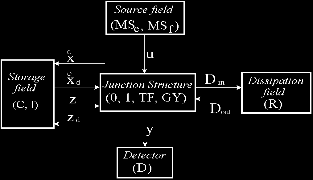
Fig. 1. Key vectors of a bond graph.
In fig. 1, ( MS , MS , ( C, I ) and ( R) denote the source, the energy storage and the e
f )
energy dissipation fields, ( D) the detector and (0,1, TF, GY ) the junction structure with transformers, TF , and gyrators, GY .
The state ( ) ∈ ℜ n
x t
and x ( t) ∈ ℜ m are composed of energy variables p( t) and q( t) d
associated with I and C elements in integral causality and derivative causality, respectively,
( ) ∈ ℜ p
u t
denotes the plant input, ( ) ∈ ℜ q
y t
the plant output, ( ) ∈ ℜ n
z t
the co-energy
vector, z ( t) ∈ ℜ m the derivative co-energy and D ( t) ∈ ℜ r and D ( t) ∈ ℜ r are a mixture d
in
out
Operational Amplifiers and Active Filters: A Bond Graph Approach
285
of e( t) and f ( t) showing the energy exchanges between the dissipation field and the junction structure (Wellstead, 1979; Sueur & Dauphin-Tanguy, 1991).
The relations of the storage and dissipation fields are,
z( t) = Fx( t) (1)
z ( t) = F x ( t) (2)
d
d
d
D ( t ) = LD t
out
in ( )
(3)
The relations of the junction structure are,
⎡ x( t)
& x ( t )
⎤
⎡
⎤ ⎡ S
S
S
S ⎤
11
12
13
14
⎢ D t
out ( )⎥
⎢
⎥ ⎢
⎥
D t
S
S
S
(4)
in ( )
=
0 ⎢
⎥
21
22
23
⎢
⎥ ⎢
⎥ ⎢ u ( t) ⎥
⎢⎣ y( t) ⎥⎦ ⎢⎣ S
S
S
0 ⎥⎦ ⎢
⎥
31
32
33
⎣ & x t
d ( ) ⎦
z ( t ) = − T
S z t
d
14
( )
(5)
The entries of S take values inside the set {0, 1
± , ± m, ± }
n where m and n are
transformer and gyrator modules; S and S are square skew-symmetric matrices and
11
22
S and S are matrices each other negative transpose. The state equation is (Wellstead,
12
21
1979; Sueur & Dauphin-Tanguy, 1991),
& x ( t ) = A x t
B u t (6)
p
( ) + p ( )
y ( t ) = C x ( t) + D u t
p
p
( )
(7)
where
1
−
A = E ( S + S MS
F (8)
p
11
12
21 )
1
−
B = E ( S + S MS
(9)
p
13
12
23 )
C = ( S + S MS
F (10)
p
31
32
21 )
D = S + S MS (11)
p
33
32
23
being
1
−
E = I +
T
S F S F
(12)
n
14
d
14
286
New Approaches in Automation and Robotics
M
( I LS ) 1−
=
−
L (13)
n
22
3. Bond graph in derivative causality assignment
We can use the Bond Graph in Derivative causality assignment (BGD) to solve directly the
problem to get
1
−
A . Suppose that A is invertible and a derivative causality assignment is
p
p
performed on the bond graph model (Gonzalez et al., 2005). From (4) the junction structure
is given by,
⎡ z( t) ⎤
⎡
J
J
J
& x( t) ⎤
⎡
⎤
11
12
13
⎢
⎥
⎢
⎥
⎢
⎥
⎢ D
t
J
J
J
D
t (14)
ind ( )⎥ =
⎢
⎥
⎢ 21
22
23 ⎥
outd ( )
⎢ y t
J
J
J
u t
d ( ) ⎥
⎢
⎥
⎢
⎥
⎢
⎥ ⎣ 31
32
33 ⎦ ⎢
( ) ⎥
⎣
⎦
⎣
⎦
where the entries of J have the same properties that S and the storage elements in (14)
have a derivative causality. Also, D and D
are defined by
ind
outd
D
( t) = L D t (15)
outd
d
ind ( )
and they depend of the causality assignment for the storage elements and that junctions
have a correct causality assignment.
From (6) to (13) and (14) we obtain,
z ( t)
*
= A x&( t)
*
+ B u t
p
p
( ) (16)
y ( t)
*
= C x&( t)
*
+ D u t
d
p
p
( )
(17)
where
*
A = J + J NJ
p
11
12
21 (18)
*
B = J + J NJ
p
13
12
23 (19)
*
C = J + J NJ
p
31
32
21 (20)
*
D = J + J NJ
p
33
32
23 (21)
being
−
N = ( I − L J
L
n
d
) 1
22
d
(22)
The state output equations of this system in integral causality are given by (6) and (7). It
follows, from (1), (6), (7), (16) and (17) that,
Operational Amplifiers and Active Filters: A Bond Graph Approach
287
*
1
A
FA−
=
p
p (23)
*
1
B
FA−
= −
B
p
p
p (24)
*
1
C
C A−
=
p
p
p (25)
*
1
D
D
C A−
=
−
B
p
p
p
p
p (26)
Considering x& ( t ) = 0 , the steady state of a LTI MIMO system defined by
1
x
A−
= −
B u
ss
p
p ss (27)
y
(
1
D
C A−
=
−
B u
ss
p
p
p
p ) ss (28)
where x
y
ss and
ss are the steady state of the state variables and the output, respectively.
In an approach of the BGD, the steady state is determined by
1
−
*
x = F B u
ss
p ss (29)
*
y = D u
ss
p ss (30)
4. A bond graph model of an operational amplifier
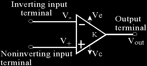
The standard operational amplifier (op-amp) symbol is shown in Fig. 2. It has two input
terminals, the inverting (-) input and the noninverting (+) input, and one output terminal.
The typical op-amp operates with two Direct Current (DC) supply voltages, one positive
and the other negative (Stanley, 1994).
Fig. 2. Operational amplifier symbol.
The complex action of the op-amp results in the amplification of the difference between the
voltages at the noninverting, V+ , and the inverting, V− , inputs by a large gain factor, K , designed open loop gain. The output voltage is,
V = K V − V
out
( + − ) (31)
288
New Approaches in Automation and Robotics
The assumptions of the ideal op-amp are (Barna & Porat, 1989): 1) The input impedance is
infinite. 2) The output impedance is zero. 3) The open loop gain is infinite. 4) Infinite
bandwidth so that any frequency signal from 0 to ∞ Hz can be amplified without
attenuation. 5) Infinite slew rate so that output voltage charges simultaneously with input
voltage charges.
The implications of the assumptions are: no current will flow either into or out of either
input terminal of the op-amp, also, the voltage at the output terminal does not charge as the
V
loading is varied and finally, from H
V − V = out
3 ,
, if we take the limit when K→∞, note
+
−
K
that V = V
+
− , which indicates that the voltages at the two input terminals are forced to be
equal in the limit.
The assumptions of an op-amp are not completely true in practice, and to be fully competent
in the analysis and design of op-amps circuits, one must be aware of the limitations.
Therefore, we propose a more realistic model applicable to DC and low frequencies based
on Bond Graph with Intregral causality assignment (BGI), since an op-amp is a multistage
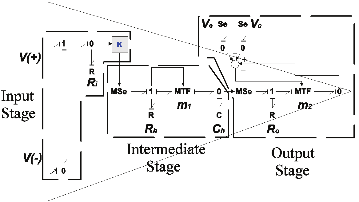
amplifier, it can be represented by Fig. 3.
Fig. 3. Bond graph model of an operational amplifier.
The individual stages used in op-amp are separately chosen to develop different amplifier
characteristics. Those amplifier characteristics which are determined by a given stage
depend on whether it functions as an input stage, intermediate stage or output stage. So, the
bond graph model of the op-amp is composed by 3 stages, which are:
•
Characteristics of the differential input stage of an operational amplifier are the most
critical factors which affect the accuracy of an op-amp in providing voltage gain. Errors
effects of following stages are reduced in significance by the gain isolation provided by
the first stage. This input stage considers the two input terminals of op-amp, the
differential input resistance, denoted as Ri , which is the resistance between the
inverting and non-inverting inputs and K is the open loop gain.
•
The intermediate stage introduces the frequency compensation of the op-amp using a
lag network. Also, using a MTF , the slew rate of the op-amp is considered.
•
Following the input and intermediate voltage gain stages of an op-amp, it is desirable to
provide impedance isolation from loads. In this way the characteristics of the gain
Operational Amplifiers and Active Filters: A Bond Graph Approach
289
stages are preserved under load, and adequate signal current is made available to the
load. In addition, the output stage provides isolation to the preceding stage and a low
output impedance to the load. This stage is formed by the output terminal, the output
resistance of the op-amp denoted as R and the adjustment of supply voltages, positive
o
voltage V
V
c and negative voltage e , are applied using a MTF element.
The usefulness of the bond graph model of an operational amplifier can be shown, applying
this model to μ 74
A 1 op-amp by Fairchild Semiconductor Corporation (Stanley, 1994;
Gayakward, 2000) and, TL 084 and OP 27 by Texas Instruments (Stanley, 1994;
Gayakward, 200