+ m RR R
o
L
i
i
2
L
i
Substituting (13), (58) (59) into (9), B is determined by,
p
⎡ R R m R
i (
2
+
o
L
⎤
2
)
1 ⎢
⎥
B =
(61)
p
1
−
Δ ⎢
( m KR R R ⎥
1
o
i
L )
⎢⎣ R
⎥
h
⎦
From (10), (13), (57), (58) and (59) the C matrix is,
p
1 ⎡ 1
−
1
⎤
C =
R R R R
m RR R
(62)
p
( + i )
⎢
o
L
2
Δ
i
L ⎥
⎣ C
Ch
⎦
Finally, substituting (13), (58) and (59) into (11), D is given by,
p
1
D =
R R R (63)
p
Δ o i L
The transfer function of a system represented in space state can be calculated by,
−
G s = C ( sI − A ) 1
( )
B + D (64)
p
n
p
p
p
Substituting (60), (61), (62) and (63) into (64), the transfer function of the op-amp integrator
of Fig. 17 is,
( 2
2
s CC R R + sCR m − Km m R R
h
h
o
o
1
1
2 )
G( s) =
L
i
(65)
2
s CC R Δ + s C R
CRR R Km m
Cm
m
h
h
(
2
Δ +
+
Δ
h
h
L
i
) 2
+
Λ
1
2
1
1
where Λ = ( R + R )(
2
R + m R .
i
o
2
L )
Considering a normal operation of the op-amp, m = m = 1 and R = 0 , we have,
1
2
o
1
−
G ( s) =
(66)
1
CC R R
⎡ C R ⎛ R
⎞
CR ⎤
1 ⎛ R
⎞
2
h
h
s
+
h
h
s
+1 + CR +
+
+1
⎢
⎜
⎟
⎥
⎜
⎟
K
⎣ K ⎝ R
K
K R
i
⎠
⎦
⎝ i
⎠
Operational Amplifiers and Active Filters: A Bond Graph Approach
303
In addition, applying lim G ( s) , the ideal transfer function, G ( s) , is determined by, 1
i
R →∞
i
K →∞
1
−
G ( s) =
i
(67)
sRC
Note that, (67) is the typical transfer function of a integral controller. However, the equation
(65) is the transfer function of a integral controller based on op-amp and considering their
internal parameters and external elements.
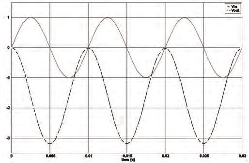
The time response of the integrator circuit using μ A 741 op-amp and R = 10Ω , C = 100μ F
and v ( t) = sin(2π f t) V where f = 1 KHz shows in Fig. 18. The output signal proves that the i
i
i
bond graph model of Fig. 18, is an integrator of the input signal.
Fig. 18. Time response of the integrator.
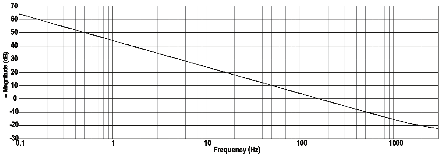
The frequency response of the integrator circuit of Fig. 17 is shown in Fig. 19. Note that (67)
is represented by Fig. 19.
Fig. 19. Frequency response of the integrator circuit.
Next section an important application of the op-amp that is an active filter in the physical
domain is proposed.
304
New Approaches in Automation and Robotics
7. Active filters using bond graph models
An electric filter is often a frequency selective circuit that passes a specified band of
frequencies and blocks or attenuates signals of frequencies outside this band. Filters may be
classified in a number of ways (Gayakward, 2000):
1. Analog or digital. Analog filters are designed to process analog signals, while digital
filters process analog signals using digital techniques.
2. Passive or active. Passive filters use resistors, capacitors and inductors in their
construction and the active filters employ transistor or op-amps in addition to resistors
and capacitors.
An active filter offers the following advantages over a passive filter: a) Gain and frequency
adjustment flexibility. b) No loading problem. c) Cost.
A filter will usually conform to one of four basic response types: low-pass, high-pass, band-
pass and band-reject.
7.1 Low-pass filter
A low-pass filter allows only low frequency signals to pass through, while suppressing
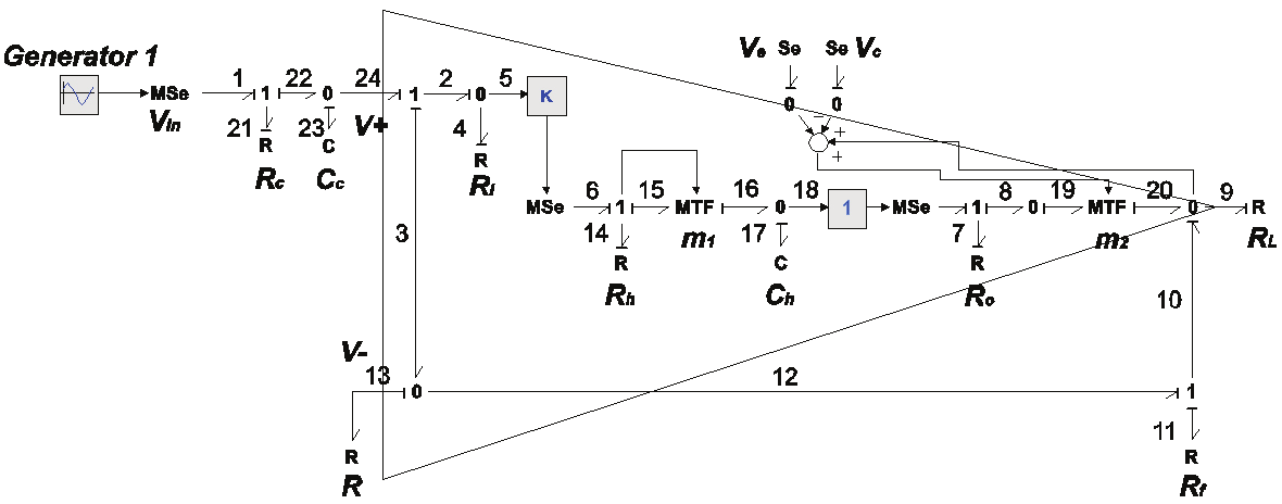
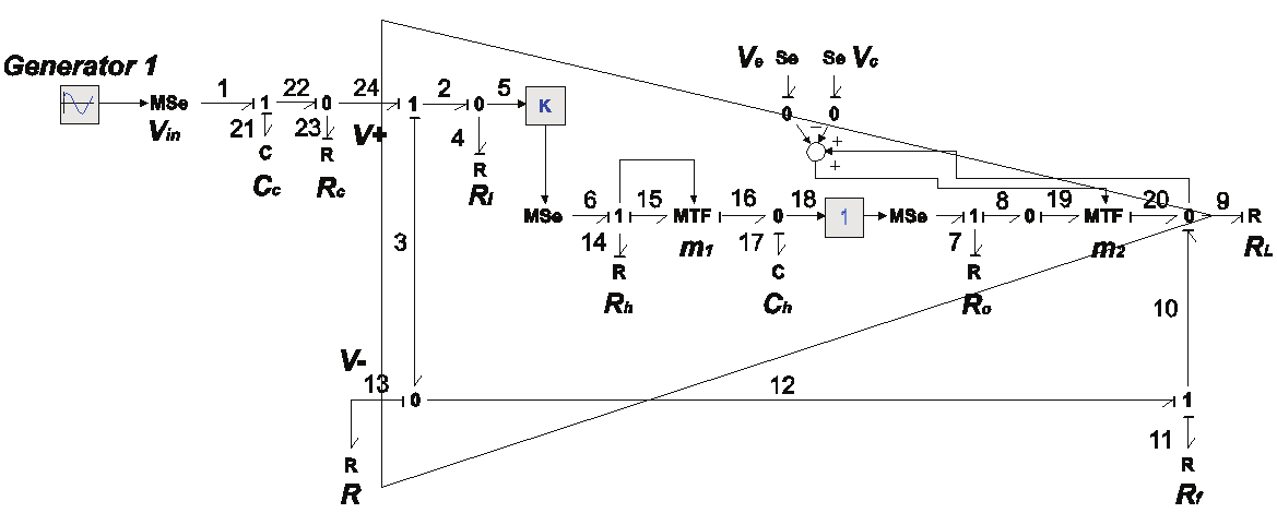
high-frequency components. The bond graph model of a low-pass filter is shown in Fig. 20.
Fig. 20. Bond graph model of a low-pass filter.
The key vectors of the bond graph of Fig. 20 are,
⎡ q ( t)⎤
⎡ f ( t)⎤
⎡ e ( t)⎤ u( t) = e ( t)
17
17
17
1
x( t) =
; & x( t) =
; z( t) =
;
⎢
⎥
⎢
⎥
⎢
⎥
⎣ q ( t)⎦
⎣ f ( t)⎦
⎣ e ( t)⎦ y( t) = e ( t)
23
23
23
9
D ( t) = [ e ( t) e ( t) e ( t)
f ( t)
f ( t)
e ( t)
e ( t) T (68)
in
4
7
9
11
13
14
21
]
D ( t) = [ f ( t)
f ( t)
f ( t)
e ( t)
e ( t)
f ( t)
f ( t) T
out
4
7
9
11
13
14
21
]
The constitutive relations of the elements are,
⎧ 1 1 ⎫
F = diag ⎨
,
⎬ (69)
⎩ C C
h
e ⎭
Operational Amplifiers and Active Filters: A Bond Graph Approach
305
⎧ 1 1 1
1
1 ⎫
L = diag ⎨ ,
,
, R , R,
,
(70)
f
⎬
⎩ R R R
R
R
i
o
L
h
c ⎭
and the junction structure is
⎡ 0 1 ⎤
⎢
⎥
⎡ 0
P
⎤
1
0
3×3
1
⎢
⎥
S = ⎢− T
⎥
P
0
0
; S = ⎢ 0
⎥
22
1
2×2
7×2
21
3×2
⎢
⎥
⎢
⎥
⎢⎣ 0
P
⎥⎦
− m
K
2×3
2
1
⎢
⎥
⎢ 0
1
− ⎥
⎣
⎦
⎡ 0
m
0⎤
⎡0 ⎤
1
6 1
S =
0
;
×
S =
(71)
12
2×4
23
⎢
⎥
⎢
⎥
⎣ 1
−
0
1⎦
⎣ 1 ⎦
S = 0
1
−
1 0
; S = S = S = S = 0
32
[ 1×3
1×2 ]
11
13
31
33
where
⎡ 0
1
− ⎤
⎢
⎥
⎡0 − K ⎤
P = m
− m ; P =
(72)
1
2
2
2
⎢
⎥
⎢
⎥
⎣0
0 ⎦
⎢⎣ 1
−
1 ⎥⎦
From (8), (13), (69), (70) and (71), the Ap matrix of the low-pass filter is,
2
⎡ − m
m m KRR R
− m K
m RK
L
i
⎤
1
1
2
1
1
−
−
⎡
⎢
R R
R
m R R
o (
+
L
f )
2
+
L
f ⎤
⎣
2
⎦
R C
Δ C
R C
Δ
⎥
C
A = ⎢ h h
h
h
h
h
⎥ (73)
p
⎢
m RR
1
−
1
⎥
2
L
−
⎡⎣( R + R R m R
R R
f ) (
2
+
+
o
L
o
L ⎤
⎢
2
)
⎦⎥
⎣
Δ C
R C
Δ C
h
c
c
h
⎦
where Δ = R [( R + R )( R + R ) + RR ]
2
+ m RR R + R + R R R
o
L
f
i
i
2 [
L (
f
i )
L
f
i ]
Substituting (70) and (71) into (13), the Bp matrix is obtained
⎡
T
1 ⎤
B = 0
(74)
p
⎢
⎥
⎣
Rc ⎦
Finally, from (10), (13), (69), (70) and (71), the Cp matrix is
306
New Approaches in Automation and Robotics
⎡ m R
RR R ⎤
2
C =
L ⎡ R R
R
R R
(75)
p
⎣ ( +
i
f ) +
⎤
⎢
L
o
Δ
i
f ⎦
⎣ C
Δ
⎥
C
h
h
⎦
and D = 0
p
From (73) to (75), and (64), and considering ideal characteristics of the op-amp, R = 0 ,
o
R = ∞ , K = ∞ and R = ∞ , the ideal transfer function of the low-pass filter, denoted by
i
L
A
R C
R
G ( s) is obtained G ( s) = CL
C
C
where A = 1 + f .
i
i
s + 1 R C
CL
R
c
C
The ideal transfer function of the low-pass filter indicates that on the pass band the gain is
almost A
f
CL and the pole of the system is located at the high cutoff frequency
h defined
1
by f =
.
h
2π C R
C
C
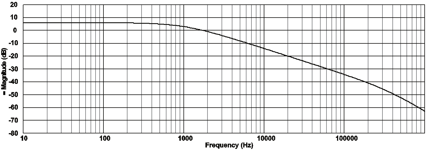
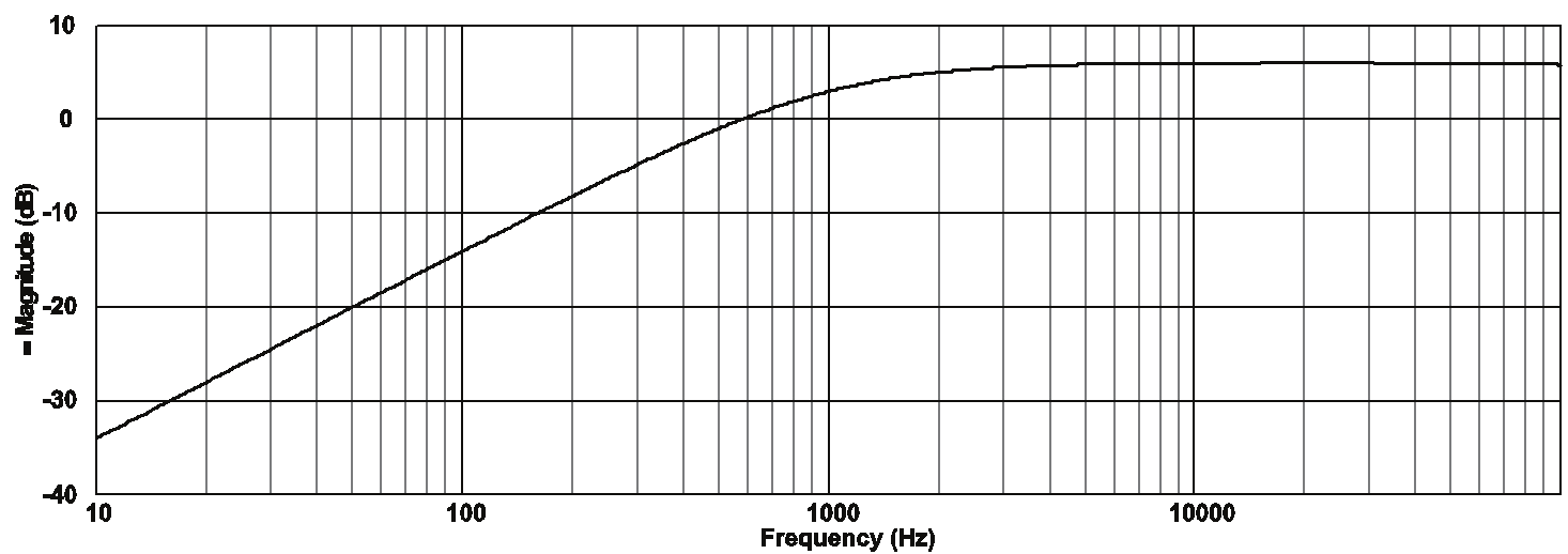
The frequency response of the low-pass filter based on bond graph model using the μA741
op-amp and considering the numerical values of the Table 3 is shown in Fig 21.
R
R
R
R
C
f
L
c
C
10 KΩ
10 KΩ
1 KΩ
15.9 KΩ
8
1 10−
×
F
Table 3. Numerical values of the low-pass filter.
Fig. 21. Frequency response of the low-pass filter.
The Fig 21 shows that f = 1 KHz . Also, we have a first order filter, because the filter has a
h
pole and the rolloff rate of the filter is 20 dB per decade.
7.2 High-pass filter
A high pass filter allows only frequencies above a certain break point to pass through. In
other words, it attenuates low frequency components. A first order high-pass filter on bond
graph model is shown in Fig. 22.
Operational Amplifiers and Active Filters: A Bond Graph Approach
307
Fig. 22. Bond graph model of a high-pass filter.
The mathematical model of the filter can be determined in the same manner that the low-
pass filter. However, for all the remaining filters of this paper, we use the software 20-sim to
know the performance of the filter on the physical domain, considering the internal
characteristics of the op-amp and the external components connected to the op-amp in order
to get the filter type.
Using the same numerical values that the low-pass filter, the frequency response of the filter
shows in Fig. 23.
Fig. 23. Frequency response of the high-pass fil