i
G =
G
G
p
∑( i−1 ⊗ 1
p− j
j )
⎪⎩
j=1
•
Evolutionary algorithm of backward iteration method
By using one of the presented approaches of the reversing recurrent equation of system (1)
formulated above, the reversing trajectory technique can be run by the following conceptual
algorithm.
1. Verify that the origin equilibrium of the system (1) is asymptotically stable i.e.
eig ( F ) < 1 .
1
2. Determine a guaranteed stable region (GSR) noted Ω0 using the theorem 1 proposed in
(Benhadj, 1996a) and presented in page 64.
3. Determine the discrete reverse model of the system (1) using the first or the second
approach.
4. Apply the reverse model for different initial states belonging to the boundary Γ0 of the
GSR Ω0.
On the Estimation of Asymptotic Stability Region of Nonlinear Polynomial Systems:
Geometrical Approaches
59
The application of the backward iteration k times on the boundary Γ0 leads to a larger
stability region Ω
Ω ⊂ Ω ⊂ ... ⊆ Ω
⊂ Ω
k such that
0
1
k −1
k .
The performance of the backward iteration algorithm depends on the used inversion
technique of the polynomial discrete model among the above two proposed approaches.
In order to compare the two formulated approaches, we propose next their implementation
on a synchronous generator second order model.
2.3 Simulation study
We consider the simplified model of a synchronous generator described by the following
second order differential equation (Willems, 1971):
2
d δ
dδ
+ a
+ sin (δ + δ −
δ
=
(11)
2
0 )
sin ( 0 ) 0
dt
dt
where δ0 is the power angle and δ is the power angle variation.
⎧ x = δ
1
The continuous state equation of the studied process for the state vector: ⎪⎨
dδ is
⎪ x =
⎩ 2
dt
given by the following couple of equation:
.
⎪⎧ x 1 = x
⎨
2
(12)
.
⎪⎩ x 2 = − ax − sin x δ
sin δ
2
( +
1
0 ) +
0
where a is the damping factor.
This nonlinear system can be approached by a third degree polynomial system:
[2]
[3]
X
= A . X + A . X
+ A . X
k +
(13)
1
1
k
2
k
3
k
⎛ 0
0 0 0⎞
⎛
0
1 ⎞
with
⎜
A
A
δ
⎟
=
,
=
1
⎜⎜
⎟⎟
sin
− cosδ
−
2
a
⎜
0
0 0 0⎟
⎝
0
⎠
⎝ 2
⎠
⎛
⎞
⎜ 0
0
⎟
and
⎜
⎟
A =
3
⎜
0 ×26 ⎟
⎜ cosδ0
⎟
⎜
0
⎟
⎝ 6
⎠
The discretization of the state equation (13) using Newton-Raphson technique (Jennings &
McKeown, 1992), (Bacha et al, 2006a) ,(Bacha et al, 2006b) with a sampling period T leads to
the following discrete state equation of the synchronous machine:
60
New Approaches in Automation and Robotics
[2]
[3]
X
=
+
+
k 1
+
1
F . X k
2
F . X k
3
F . X k
(14)
⎛
0
0 0 0⎞
⎛
1
T ⎞
with
⎜
F
F
T
δ
⎟
=
,
=
1
⎜⎜
⎟⎟
.sin
− T cosδ
1 − aT
⎜
0
2
0 0 0⎟
⎝
0
⎠
⎝
2
⎠
⎛
⎞
⎜
0
0
⎟
and
⎜
⎟
F =
3
⎜
02×6 ⎟
⎜ T.cos δ0
⎟
⎜
0
⎟
⎝
6
⎠
⎧δ = 412
.
0
0
With the following parameters: ⎪⎨ a = 5
.
0
⎪⎩ T = 05
.
0
one obtains the following numerical values of the matrices Fi , i=1, 2, 3.
⎛
1
0.05 ⎞
⎛
0
0 0 0⎞
F = ⎜
⎟ , F =
1
2
0.0458
−
0.975
⎜0.0076 0 0 0⎟
⎝
⎠
⎝
⎠
⎛ 0
0
⎞
⎜
⎟
F =
3
⎜
02×6 ⎟
⎜
⎟
⎝0.01 0
⎠
One can easily verify that the equilibrium Xe=0 is asymptotically stable since we have
eig ( F < 1 .
1 )
Our aim now is the estimation of a local domain of stability of the origin equilibrium Xe=0.
For this goal, we make use of the backward iteration technique with the proposed inversion
algorithms of the direct system (14) applied from the boundary Γ0 of the ball Ω0 centred in
the origin and of radius R0=0.42 which is a guaranteed stability region (GSR) that
characterized the method developed in (Benhadj, 1996a).
•
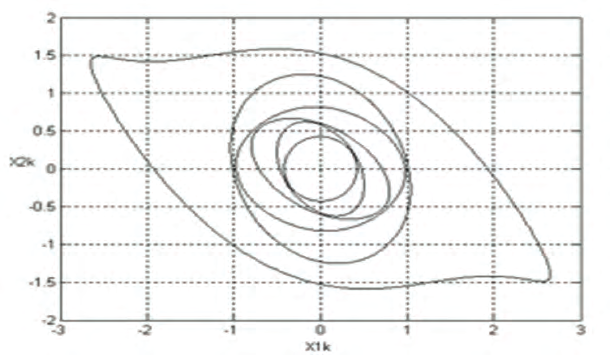
Domain of stability obtained by using the first approach of discrete model
inversion :
The implementation of the first approach of the discrete model inversion described by
equation (4) leads, after running 2000 iterations, to the region of stability represented in the
figure 1.
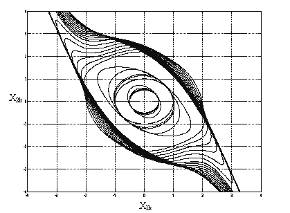
Figure 2 represents the stability domain of the discrete system (14) obtained after running
the backward iteration based on the inversion model (4) 50000 times.
It is clear that the domain obtained after 50000 iterations is larger than that obtained after
2000 iterations and it is included in the exact stability domain of the studied system, which
reassures the availability of the first proposed approach of the backward iteration
formulation.
On the Estimation of Asymptotic Stability Region of Nonlinear Polynomial Systems:
Geometrical Approaches
61
Fig. 1. RAS of discrete synchronous generator model obtained after 2000 backward iterations
based on the first proposed approach
Fig. 2. RAS of discrete synchronous generator model obtained after 50000 backward
iterations based on the first proposed approach.
•
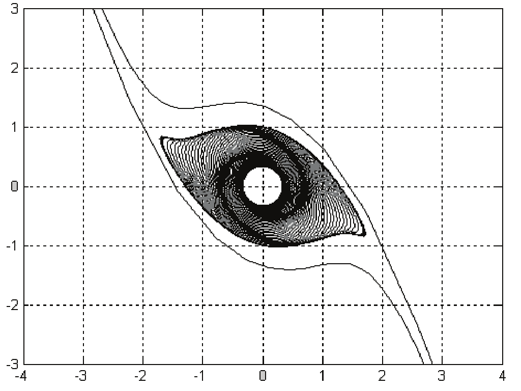
Domain of stability obtained by using the second approach of discrete model
inversion
When applying the discrete backward iteration formulated by using the reverse model (8)
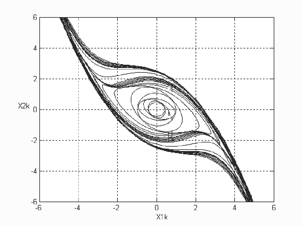
we obtain the stability domain shown in figure 3 after 1000 iterations and the domain
presented in figure 4 after 50000 iterations.
In figure 4 it seems that the stability domain estimated by the second approach of backward
iteration is larger and more precise than that obtained by the first approach. The reached
stability domain represents almost the entire domain of stability, which shows the efficiency
of the second approach of the backward iteration, particularly when the order of the studied
system is not very high as a second order system.
62
New Approaches in Automation and Robotics
Fig. 3. RAS of discrete synchronous generator model obtained after 1000 backward
iterations based on the second proposed approach
Fig. 4. RAS of discrete synchronous generator model obtained after 50000 backward
iterations based on the second proposed approach
2.4 Conclusion
In this work, the extension of the reversing trajectory concept for the estimation of a region
of asymptotic stability of nonlinear discrete systems has been investigated.
The polynomial nonlinear systems have been particularly considered.
Since the reversing trajectory method, also called backward iteration, is based on the
inversion of the direct discrete model, two dissimilar approaches have been proposed in this
work for the formulation of the reverse of a discrete polynomial system.
The application of the backward iteration with both proposed approaches starting from the
boundary of an initial guaranteed stability region allows to an important enlargement of the
searched stability domain. In the particular case of the second order systems, the studied
technique can lead to the entire domain of stability.
The simulation of the developed algorithms on a second order model of a synchronous
generator has shown the validity of the two approximation ideas with a little superiority of
the second approach of the discrete model inversion, since the RAS obtained by this last one
is larger and more precise than the one yielded by the first approximation approach.
On the Estimation of Asymptotic Stability Region of Nonlinear Polynomial Systems:
Geometrical Approaches
63
3. Technique of a guaranteed stability domain determination
In this part we consider a new advanced approach of estimating a large asymptotic stability
domain for discrete time nonlinear polynomial system. Based on the Kronecker product
(Benhadj Braiek, 1996a; Benhadj Braiek, 1996b) and the Grownwell-bellman lemma for the
estimation of a guaranteed region of stability; the proposed method permits to improve
previous results in this field of research.
3.1 Description of the studied systems
We consider the discrete nonlinear systems described by a state equation of the following
form
q
X ( k + 1) = F( x( k)) = ∑
[ i
A X ] ( k)
(15)
i
i= 1
where k is the discrete time variable,
n
X ( k) ∈ ℜ is the state vector, [ ]
X i ( k) designates the i-
th Kronecker power of the vector X ( k ) and A , i = 1,K, q are (
i
n × n ) matrices. The
i
system (15) can also be written in the following form:
X ( k + )
1 = M ( X ( k)). X ( k)
(16)
where:
q
M ( X ( k)) = A + ∑ A (
[ j− ]
1
I ⊗ X
( X ( k))
(17)
1
j
n
j=2
where ⊗ is the Kronecker product (Benhadj Braiek, 1996a; Benhadj Braiek, 1996b).
Assumption 1: The linear part of the discrete systems (15) is asymptotically stable i.e. all the
eigenvalues of the matrix are of module little than 1.
3.2 Guaranteed stability region
Our purpose is to determine a sufficient domain Ω 0 of the initial conditions variation, in
which the asymptotic stability of system (15) is guaranteed, according to the following
definition:
X
∀
∈ Ω
X , ,
∈ ℜ ∀
0
0
( k k X
0
0 )
k
and
lim X ( k, k , X ) = 0
(18)
0
0
k →+∞
where X ( k, k , X ) designates the solution of the nonlinear recurrent equation (15) with 0
0
the initial condition X ( k ) = X .
0
0
The stability domain that we propose is considered as a ball of radius R 0 and of centre the
origin X = 0 i.e.,
Ω = X ∈ ℜ ; X
< R (19)
0
{
n
0
0
0 }
64
New Approaches in Automation and Robotics
the radius R 0 is called the stability radius of the system (15).
A simple domain ensuring the stability of the system (15) is defined by the following
theorem (Benhadj Braiek, 1996b).
Theorem 1. Consider the discrete system (15) satisfying the assumption 1, and let c and α
the positive numbers verifyingα ∈ ]0 1[,
k − k
−
0
k k 0
A
≤ cα
∀ k ≥ k
(20)
1
0
Then this system is asymptotically stable on the domain Ω0 defined in (19) with R 0 the
unique positive solution of the following equation:
q
α
k 1
1 −
∑
−
γ R
−
= 0
(21)
k
0
k = 2
c
where γ , k = 2,..., q denote :
k
k
γ
c 1
−
=
A
k
k
(22)
Furthermore the stability is exponentially.
Proof. The equation (15) can be written as:
X ( k + )
1 = A X ( k) + h( X ( k)) X ( k)
(23)
1
with
q
h( X ( k)) = ∑
[ j−
A ( I ⊗
1
X
] ( k))
(24)
j
n
j= 2
Let us consider that:
∀ k ≥ k , X ( k) ≤ R
(25)
0
then we have, using the matrix norm property of the Kronecker product
h( X ( k)) ≤ λ( R)
(26)
with:
q
j− 1
λ( R) = ∑ A R
(27)
j
j= 2
By using the lemma 1(see the appendix), we have:
X ( k) ≤ c(α + cλ( R)) k− k 0 X ( k )
(28)
0
On the Estimation of Asymptotic Stability Region of Nonlinear Polynomial Systems:
Geometrical Approaches
65
with g( X ) = h( X ) X ,we have g( X ) ≤ λ( R) X .
Then, if:
α
λ
−
( R < 1
)
(29)
c
Now, to ensure the hypothesis (25) it is sufficient to have (from (21)):
R
c X ( k ) ≤ R
X ( k ) ≤ R
1
=
0
1 or
0
0
(30)
c
R satisfies the equation (29) implies that R satisfies the equation (21) of the theorem 1.
1
0
3.3 Enlargement of the guaranteed stability region (GSR)
Our object in this section is to enlarge the Guaranteed Stability Region Ω 0 characterized in
the section 3.2. For this goal, we consider the boundary Γ 0 of the obtained GSR of radius R0.
Let Xi0 be a point belonging in Γ 0, and Xik the image of Xi0 by the F( . ) function characterizing the considered system, k times.
i
k
X = F ( i
X (31)
k
0 )
Xik is then a point belonging in the stability domain Ω0;
i
X &