Basic Numerical Integration with MATLAB
This chapter essentially deals with the problem of computing the area under a curve. First, we will employ a basic approach and form trapezoids under a curve. From these trapezoids, we can calculate the total area under a given curve. This method can be tedious and is prone to errors, so in the second half of the chapter, we will utilize a built-in MATLAB function to carry out numerical integration.
There are various methods to calculating the area under a curve, for example, Rectangle Method, Trapezoidal Rule and Simpson's Rule. The following procedure is a simplified method.
Consider the curve below:
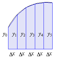
Each segment under the curve can be calculated as follows:

Therefore, if we take the sum of the area of each trapezoid, given the limits, we calculate the total area under a curve. Consider the following example.
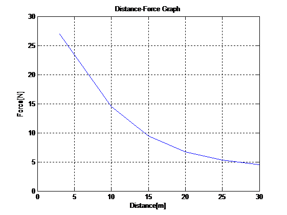
Given the following data, plot an x-y graph and determine the area under a curve between x=3 and x=30
| Index | x [m] | y [N] |
|---|---|---|
| 1 | 3 | 27.00 |
| 2 | 10 | 14.50 |
| 3 | 15 | 9.40 |
| 4 | 20 | 6.70 |
| 5 | 25 | 5.30 |
| 6 | 30 | 4.50 |
First, let us enter the data set. For x, issue the following command x=[3,10,15,20,25,30];. And for y, y=[27,14.5,9.4,6.7,5.3,4.5];. If yu type in [x',y'], you will see the following tabulated result. Here we transpose row vectors with ' and displaying them as columns:
ans =

    3.0000   27.0000
   10.0000   14.5000
   15.0000    9.4000
   20.0000    6.7000
   25.0000    5.3000
   30.0000    4.5000
Compare the data set above with the given information in the question.
To plot the data type the following:
plot(x,y),title('Distance-Force Graph'),xlabel('Distance[m]'),ylabel('Force[N]'),gridThe following figure is generated:
To compute dx for consecutive x values, we will use the index for each x value, see the given data in the question.:
dx=[x(2)-x(1),x(3)-x(2),x(4)-x(3),x(5)-x(4),x(6)-x(5)];
dy is computed by the following command:
dy=[0.5*(y(2)+y(1)),0.5*(y(3)+y(2)),0.5*(y(4)+y(3)),0.5*(y(5)+y(4)),0.5*(y(6)+y(5))];
dx and dy can be displayed with the following command: [dx',dy']. The result will look like this:
[dx',dy']

ans =

    7.0000   20.7500
    5.0000   11.9500
    5.0000    8.0500
    5.0000    6.0000
    5.0000    4.9000
Our results so far are shown below
| x [m] | y [N] | dx [m] | dy [N] |
|---|---|---|---|
| 3 | 27.00 | ||
| 10 | 14.50 | 7.00 | 20.75 |
| 15 | 9.40 | 5.00 | 11.95 |
| 20 | 6.70 | 5.00 | 8.05 |
| 25 | 5.30 | 5.00 | 6.00 |
| 30 | 4.50 | 5.00 | 4.90 |
If we multiply dx by dy, we find da for each element under the curve. The differential area da=dx*dy, can be computed using the 'term by term multiplication' technique in MATLAB as follows:
da=dx.*dy

da =

  145.2500   59.7500   40.2500   30.0000   24.5000
Each value above represents an element under the curve or the area of trapezoid. By taking the sum of array elements, we find the total area under the curve.
sum(da)

ans =

  299.7500
The following illustrates all the steps and results of our MATLAB computation.
| x [m] | y [N] | dx [m] | dy [N] | dA [Nm] |
|---|---|---|---|---|
| 3 | 27.00 | |||
| 10 | 14.50 | 7.00 | 20.75 | 145.25 |
| 15 | 9.40 | 5.00 | 11.95 | 59.75 |
| 20 | 6.70 | 5.00 | 8.05 | 40.25 |
| 25 | 5.30 | 5.00 | 6.00 | 30.00 |
| 30 | 4.50 | 5.00 | 4.90 | 24.50 |
| 299.75 |
Sometimes it is rather convenient to use a numerical approach to solve a definite integral. The trapezoid rule allows us to approximate a definite integral using trapezoids.
trapz CommandZ = trapz(Y) computes an approximation of the integral of Y using the trapezoidal method.
Now, let us see a typical problem.
Given
 ,
an analytical solution would produce 39. Use trapz command and solve it
,
an analytical solution would produce 39. Use trapz command and solve it
Initialize variable x as a row vector, from 2 with increments of 0.1 to 5: x=2:.1:5;
Declare variable y as y=x^2;. Note the following error prompt: ??? Error using ==> mpower
Inputs must be a scalar and a square matrix. This is because x is a vector quantity and MATLAB is expecting a scalar input for y. Because of that, we need to compute y as a vector and to do that we will use the dot operator as follows: y=x.^2;. This tells MATLAB to create vector y by taking each x value and raising its power to 2.
Now we can issue the following command to calculate the first area, the output will be as follows:
area1=trapz(x,y)

area1 =

   39.0050
Notice that this numerical value is slightly off. So let us increase the number of increments and calculate the area again:
x=2:.01:5;
y=x.^2;
area2=trapz(x,y)

area2 =

   39.0001
Yet another increase in the number of increments:
x=2:.001:5;
y=x.^2;
area3=trapz(x,y)

area3 =

   39.0000
Determine the value of the following integral:

Initialize variable x as a row vector, from 0 with increments of pi/100 to pi: x=0:pi/100:pi;
Declare variable y as y=sin(x);
Issue the following command to calculate the first area, the output will be as follows:
area1=trapz(x,y)

area1 =

    1.9998
let us increase the increments as above:
x=0:pi/1000:pi;
y=sin(x);
area2=trapz(x,y)

area2 =

2.0000In its simplest form, numerical integration involves calculating the areas of segments that make up the area under a curve,
MATLAB has built-in functions to perform numerical integration,
Z = trapz(Y) computes an approximation of the integral of Y using the trapezoidal method.
Problem Set for Numerical Integration with MATLAB
Let the function y defined by y=cos(x) . Plot this function over the interval [-pi,pi]. Use numerical integration techniques to estimate the integral of y over [0, pi] and over [-pi,pi].
Plotting:
x=-pi:pi/100:pi;
y=cos(x);
plot(x,y),title('Graph of y=cos(x)'),xlabel('x'),ylabel('y'),grid
Area calculation 1:
>> x=0:pi/100:pi;
>> y=cos(x);
>> area1=trapz(x,y)

area1 =

  1.1796e-016
Area calculation 2:
>> x=-pi:pi/100:pi;
>> y=cos(x);
>> area2=trapz(x,y)

area2 =

  1.5266e-016
Let the function y defined by y=0.04x2−2.13x+32.58 . Plot this function over the interval [3,30]. Use numerical integration techniques to estimate the integral of y over [3,30].
Plotting:
>> x=3:.1:30;
>> y=0.04*(x.^2)-2.13.*x+32.58;
>> plot(x,y), title('Graph of ...
y=.04*(x^2)-2.13*x+32.58'),xlabel('x'),ylabel('y'),grid
Area calculation:
>> area=trapz(x,y)

area =

  290.3868
A 2000-liter tank is full of lube oil. It is known that if lube oil is drained from the tank, the mass flow rate will decrease from the maximum when the tank level is at the highest. The following data were collected when the tank was drained.
| Time [min] | Mass Flow [kg/min] |
|---|---|
| 0 | 50.00 |
| 5 | 48.25 |
| 10 | 46.00 |
| 15 | 42.50 |
| 20 | 37.50 |
| 25 | 30.50 |
| 30 | 19.00 |
| 35 | 9.00 |
Write a script to estimate the amount of oil drained in 35 minutes.
clc
t=linspace(0,35,8)                  % Data entry for time [min]
m=[50 48.25 46 42.5 37.5 30.5 19 9] % Data entry for mass flow [kg/min]
% Calculate time intervals
dt=[t(2)-t(1),t(3)-t(2),t(4)-t(3),...
t(5)-t(4),t(6)-t(5),t(7)-t(6),t(8)-t(7)]
% Calculate mass out
dm=[0.5*(m(2)+m(1)),0.5*(m(3)+m(2)),0.5*(m(4)+m(3)),0.5*(m(5)+...
m(4)),0.5*(m(6)+m(5)),0.5*(m(7)+m(6)),0.5*(m(8)+m(7))]
% Calculate differential areas
da=dt.*dm;
% Tabulate time and mass flow
[t',m']
% Tabulate time intervals, mass out and differential areas
[dt',dm',da']
% Calculate the amount of oil drained [kg] in 35 minutes
Oil_Drained=sum(da)
The output is:
ans =

         0   50.0000
    5.0000   48.2500
   10.0000   46.0000
   15.0000   42.5000
   20.0000   37.5000
   25.0000   30.5000
   30.0000   19.0000
   35.0000    9.0000


ans =

    5.0000   49.1250  245.6250
    5.0000   47.1250  235.6250
    5.0000   44.2500  221.2500
    5.0000   40.0000  200.0000
    5.0000   34.0000  170.0000
    5.0000   24.7500  123.7500
    5.0000   14.0000   70.0000


Oil_Drained =

  1.2663e+003
A gas is expanded in an engine cylinder, following the law PV1.3=c. The initial pressure is 2550 kPa and the final pressure is 210 kPa. If the volume at the end of expansion is 0.75 m3, compute the work done by the gas.