This module is part of the collection, A First Course in Electrical and Computer Engineering. The LaTeX source files for this collection were created using an optical character recognition technology, and because of this process there may be more errors than usual. Please contact us if you discover any errors.
Phasors! For those who understand them, they are of incomparable value for the study of elementary and advanced topics. For those who misunderstand them, they are a constant source of confusion and are of no apparent use. So, let's understand them.
The conceptual leap from the complex number ejθ to the phasor ej(ωt+θ) comes in "Phasor Representation of Signals". Take as long as necessary to understand every geometrical and algebraic nuance. Write the MATLAB program in "Exercise 6" to fix the key ideas once and for all. Then use phasors to study beating between tones, multiphase power, and Lissajous figures in "Beating between Tones" through "Lissajous Figures". We usually conduct a classroom demonstration of beating between tones using two phase-locked sources, an oscilloscope, and a speaker. We also demonstrate Lissajous figures with this hardware.
"Sinusoidal Steady State and the Series RLC Circuit" and Light Scattering by a Slit" on sinusoidal steady state and light scattering are too demanding for freshmen but are right on target for sophomores. These sections may be covered in a sophomore course (or a supplement to a sophomore course) or skipped in a freshman course without consequence.
In the numerical experiment in "Numerical Experiment (Interference Patterns)", students compute and plot interference patterns for two sinusoids that are out of phase.
In engineering and applied science, three test signals form the basis for our study of electrical and mechanical systems. The impulse is an idealized signal that models very short excitations (like current pulses, hammer blows, pile drives, and light flashes). The step is an idealized signal that models excitations that are switched on and stay on (like current in a relay that closes or a transistor that switches). The sinusoid is an idealized signal that models excitations that oscillate with a regular frequency (like AC power, AM radio, pure musical tones, and harmonic vibrations). All three signals are used in the laboratory to design and analyze electrical and mechanical circuits, control systems, radio antennas, and the like. The sinusoidal signal is particularly important because it may be used to determine the frequency selectivity of a circuit (like a superheterodyne radio receiver) to excitations of different frequencies. For this reason, every manufacturer of electronics test equipment builds sinusoidal oscillators that may be swept through many octaves of Orequency. (Hewlett-Packard was started in 1940 with the famous HP audio oscillator.)
In this chapter we use what we have learned about complex numbers and the function ejθ to develop a phasor calculus for representing and ma- nipulating sinusoids. This calculus operates very much like the calculus we developed in "Complex Numbers" and "The Functions ex and ejθ" for manipulating complex numbers. We ap- ply our calculus to the study of beating phenomena, multiphase power, series RLC circuits, and light scattering by a slit.
This module is part of the collection, A First Course in Electrical and Computer Engineering. The LaTeX source files for this collection were created using an optical character recognition technology, and because of this process there may be more errors than usual. Please contact us if you discover any errors.
There are two key ideas behind the phasor representation of a signal:
a real, time-varying signal may be represented by a complex, time-varying signal; and
a complex, time-varying signal may be represented as the product of a complex number that is independent of time and a complex signal that is dependent on time.
Let's be concrete. The signal
illustrated in Figure 3.1, is a cosinusoidal signal with amplitude A, frequency
ω, and phase φ. The amplitude A characterizes the peak-to-peak swing of 2A,
the angular frequency ω characterizes the period  between negative-
to-positive zero crossings (or positive peaks or negative peaks), and the phase
φ characterizes the time
between negative-
to-positive zero crossings (or positive peaks or negative peaks), and the phase
φ characterizes the time  when the signal reaches its first peak. With
τ so defined, the signal x(t) may also be written as
when the signal reaches its first peak. With
τ so defined, the signal x(t) may also be written as
When τ is positive, then τ is a “time delay” that describes the time (greater
than zero) when the first peak is achieved. When τ is negative, then τ is a
“time advance” that describes the time (less than zero) when the last peak
was achieved. With the substitution  we obtain a third way of writing
x(t):
we obtain a third way of writing
x(t):

In this form the signal is easy to plot. Simply draw a cosinusoidal wave with amplitude A and period T; then strike the origin (t=0) so that the signal reaches its peak at τ. In summary, the parameters that determine a cosinusoidal signal have the following units:
A, arbitrary (e.g., volts or meters/sec, depending upon the application)
ω, in radians/sec (rad/sec)
T, in seconds (sec)
φ, in radians (rad)
τ, in seconds (sec)
Show that  is “periodic with period
T,"
meaning that x(t+mT)=x(t) for all integer
m.
is “periodic with period
T,"
meaning that x(t+mT)=x(t) for all integer
m.
The inverse of the period
T
is called the “temporal frequency”
of the cosinusoidal signal and is given the symbol
f
; the units of  are
(seconds)–1 or hertz (Hz). Write x(t) in terms of
f
. How is f related to ω
?
Explain why
f
gives the number of cycles of x(t) per second.
are
(seconds)–1 or hertz (Hz). Write x(t) in terms of
f
. How is f related to ω
?
Explain why
f
gives the number of cycles of x(t) per second.
Sketch the function  versus
t
. Repeat
for
versus
t
. Repeat
for  and
and  . For each
function, determine A,ω,T,f,φ, and
τ
. Label your sketches carefully.
. For each
function, determine A,ω,T,f,φ, and
τ
. Label your sketches carefully.
The signal x(t)=Acos(ωt+φ) can be represented as the real part of a complex number:

We call Aejφejωt the complex representation of x(t) and write
meaning that the signal x(t) may be reconstructed by taking the real part of Aejφejωt. In this representation, we call Aejφ the phasor or complex amplitude representation of x(t) and write
meaning that the signal x(t) may be reconstructed from Aejφ by multiplying with ejωt and taking the real part. In communication theory, we call Aejφ the baseband representation of the signal x(t).
For each of the signals in Problem 3.3, give the corresponding phasor representation Aejφ.
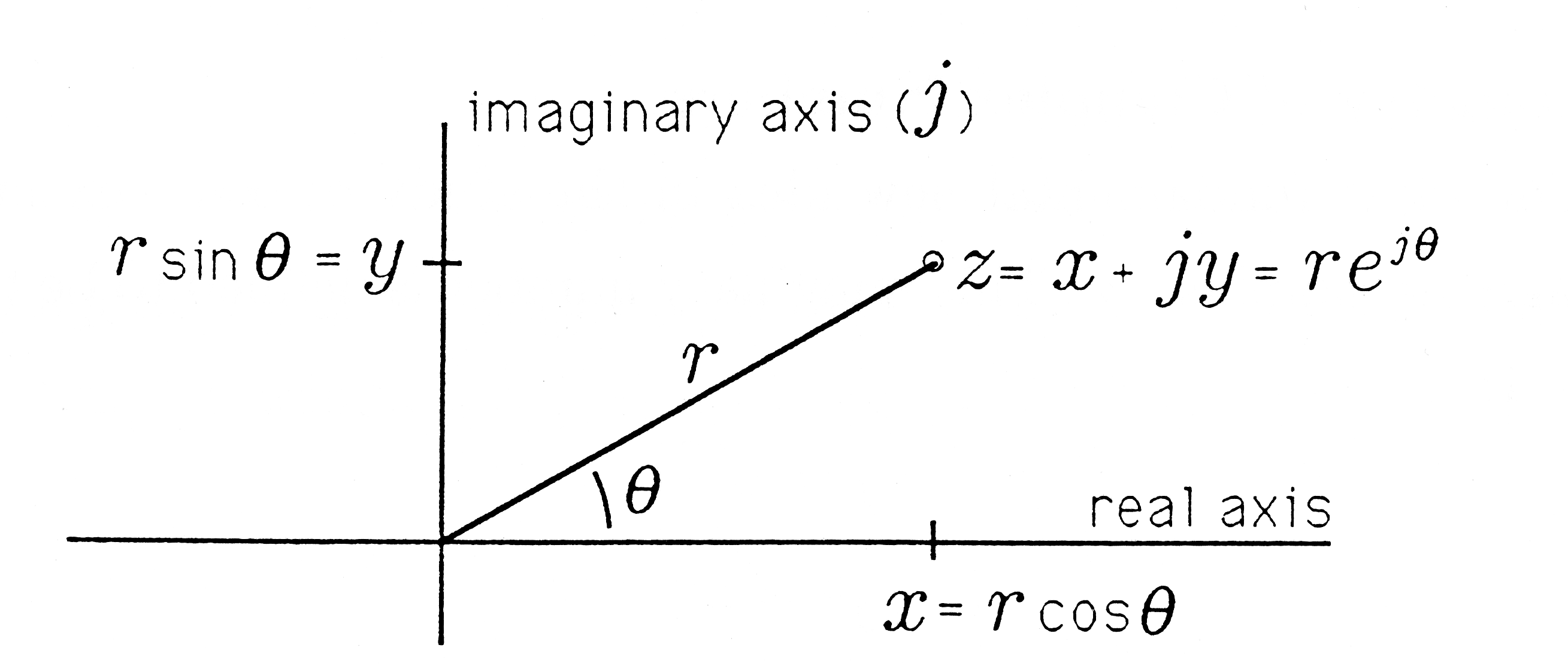
Geometric Interpretation. Let's call
the complex representation of the real signal Acos(ωt+φ). At t=0, the complex representation produces the phasor
This phasor is illustrated in Figure 3.2. In the figure, φ is approximately  If we let
t
increase to time
t1, then the complex representation produces the phasor
If we let
t
increase to time
t1, then the complex representation produces the phasor
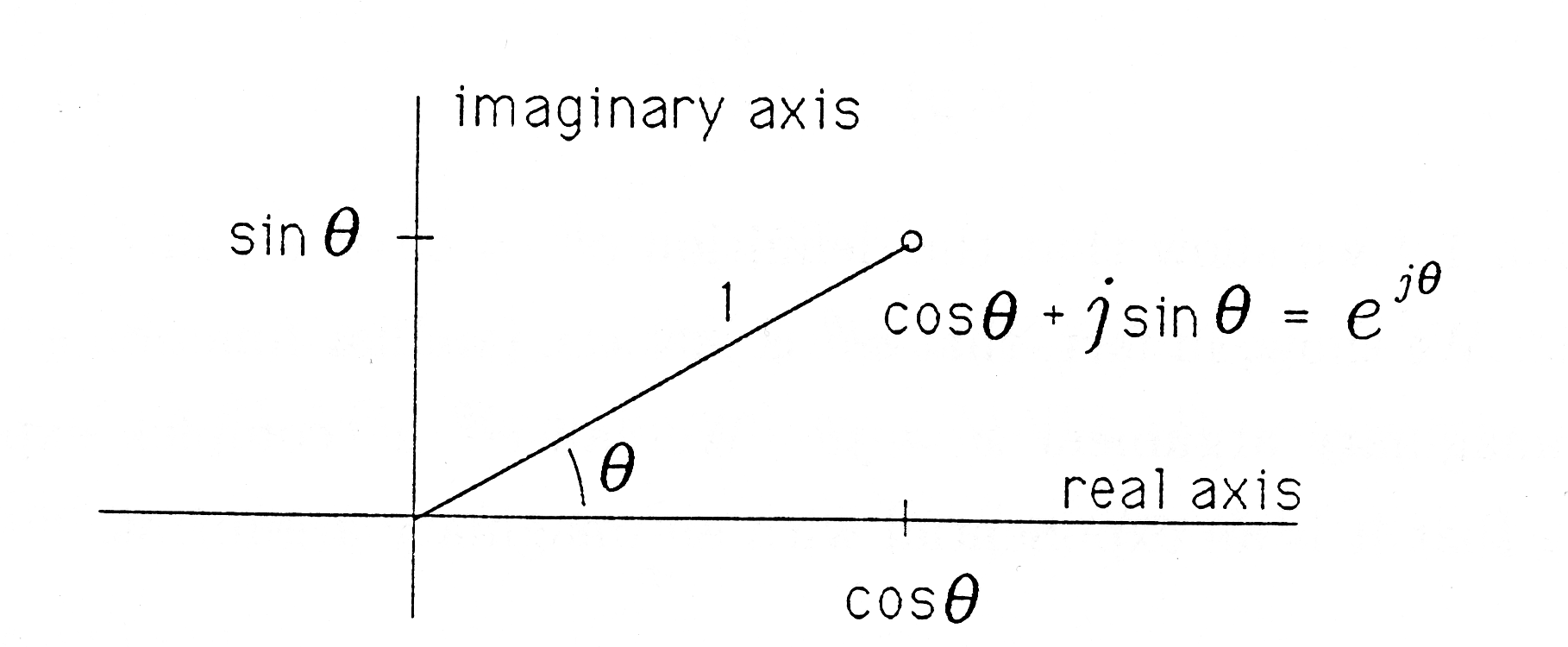
We know from our study of complex numbers that ejωt1 just rotates the phasor
Aejφ through an angle of ωt1 ! See Figure 3.2. Therefore, as we run t from 0,
indefinitely, we rotate the phasor Aejφ indefinitely, turning out the circular
trajectory of Figure 3.2. When  then ejωt=ej2π=1. Therefore,
every
then ejωt=ej2π=1. Therefore,
every  seconds, the phasor revisits any given position on the circle of
radius A. We sometimes call Aejφejωt a rotating phasor whose rotation rate
is the frequency
ω
:
seconds, the phasor revisits any given position on the circle of
radius A. We sometimes call Aejφejωt a rotating phasor whose rotation rate
is the frequency
ω
:

This rotation rate is also the frequency of the cosinusoidal signal Acos(ωt+φ).
In summary, Aejφejωt is the complex, or rotating phasor, representation of the signal Acos(ωt+φ). In this representation, ejωt rotates the
phasor Aejφ through angles ωt at the rate
ω
. The real part of the complex
representation is the desired signal Acos(ωt+φ). This real part is read off the
rotating phasor diagram as illustrated in Figure 3.3. In the figure, the angle
φ is about  . As we become more facile with phasor representations, we
will write
. As we become more facile with phasor representations, we
will write  and call Xejωt the complex representation and X
the phasor representation. The phasor
X
is, of course, just the phasor Aejφ.
and call Xejωt the complex representation and X
the phasor representation. The phasor
X
is, of course, just the phasor Aejφ.
Sketch the imaginary part of Aejφejωt to show that this is Asin(ωt+φ). What do we mean when we say that the real and imaginary parts of Aejφejωt are "90∘ out of phase"?