3. Burrus, C. Sidney and Gopinath, Ramesh A. and Guo, Haitao. (1998). Introduction to Wavelets
and the Wavelet Transform. Upper Saddle River, NJ: Prentice Hall.
4. Burrus, C. S. and Parks, T. W. (1985). DFT/FFT and Convolution Algorithms. New York: John
Wiley & Sons.
5. Bracewell, R. N. (1985). The Fourier Transform and Its Applications. (Third). New York:
McGraw-Hill.
6. Burrus, C. Sidney. (1997, July). Wavelet Based Signal Processing: Where are We and Where
are We Going?, Plenary Talk. In Proceedings of the International Conference on Digital
Signal Processing. (Vol. I, p. 3–5). Santorini, Greece
7. Churchill, R. V. and Brown, J. W. (1984). Introduction to Complex Variables and Applications.
(fourth). New York: McGraw-Hill.
8. Cohen, A. and Daubechies, I. and Feauveau, J. C. (1992). Biorthogonal Bases of Compactly
Supported Wavelets. Communications on Pure and Applied Mathematics, 45, 485–560.
9. DSP Committee, (Ed.). (1979). Digital Signal Processing II, selected reprints. New York:
9. DSP Committee, (Ed.). (1979). Digital Signal Processing II, selected reprints. New York:
IEEE Press.
10. Daubechies, Ingrid. (1988, November). Orthonormal Bases of Compactly Supported Wavelets.
Communications on Pure and Applied Mathematics, 41, 909–996.
11. Daubechies, Ingrid. (1992). Ten Lectures on Wavelets. [Notes from the 1990 CBMS-NSF
Conference on Wavelets and Applications at Lowell, MA]. Philadelphia, PA: SIAM.
12. Daubechies, Ingrid. (1996, April). Where Do Wavelets Comre From? – A Personal Point of
View. Proceedings of the IEEE, 84(4), 510–513.
13. Donoho, David L. (1993, December). Unconditional Bases are Optimal Bases for Data
Compression and for Statistical Estimation. [Also Stanford Statistics Dept. Report TR-410,
Nov. 1992]. Applied and Computational Harmonic Analysis, 1(1), 100–115.
14. Donoho, David L. (1995, May). De-Noising by Soft-Thresholding. [also Stanford Statistics
Dept. report TR-409, Nov. 1992]. IEEE Transactions on Information Theory, 41(3), 613–627.
15. Elliott, D. F. and Rao, K. F. (1982). Fast Transforms: Algorithms, Analyses and Applications.
New York: Academic Press.
16. Freeman, H. (1965). Discrete Time Systems. New York: John Wiley & Sons.
17. Hubbard, Barbara Burke. (1996). The World According to Wavelets. [Second Edition 1998].
Wellesley, MA: A K Peters.
18. Moler, Cleve and Little, John and Bangert, Steve. (1989). Matlab User's Guide. South Natick,
MA: The MathWorks, Inc.
19. Misiti, Michel and Misiti, Yves and Oppenheim, Georges and Poggi, Jean-Michel. (1996).
Wavelet Toolbox User's Guide. Natick, MA: The MathWorks, Inc.
20. Oppenheim, A. V. and Schafer, R. W. (1989). Discrete-Time Signal Processing. Englewood
Cliffs, NJ: Prentice-Hall.
21. Papoulis, A. (1962). The Fourier Integral and Its Applications. McGraw-Hill.
22. Rabiner, L. R. and Gold, B. (1975). Theory and Application of Digital Signal Processing.
Englewood Cliffs, NJ: Prentice-Hall.
23. Steffen, P. and Heller, P. N. and Gopinath, R. A. and Burrus, C. S. (1993, December). Theory
of Regular -Band Wavelet Bases. [Special Transaction issue on wavelets; Rice contribution
also in Tech. Report No. CML TR-91-22, Nov. 1991.]. IEEE Transactions on Signal
Processing, 41(12), 3497–3511.


24. Strang, Gilbert and Nguyen, T. (1996). Wavelets and Filter Banks. Wellesley, MA: Wellesley–
Cambridge Press.
25. Sweldens, Wim. (1996, April). Wavelets: What Next? Proceedings of the IEEE, 84(4), 680–
685.
26. Vetterli, Martin and Kovačević, Jelena. (1995). Wavelets and Subband Coding. Upper Saddle
River, NJ: Prentice–Hall.
5.7. Efficiency of Frequency-Domain Filtering*
To determine for what signal and filter durations a time- or frequency-domain implementation
would be the most efficient, we need only count the computations required by each. For the time-
domain, difference-equation approach, we need
. The frequency-domain approach requires
three Fourier transforms, each requiring
computations for a length- K FFT, and the
multiplication of two spectra ( 6 K computations). The output-signal-duration-determined length
must be at least Nx+ q . Thus, we must compare
Exact analytic
evaluation of this comparison is quite difficult (we have a transcendental equation to solve).
Insight into this comparison is best obtained by dividing by Nx .
With this manipulation, we are evaluating the number of
computations per sample. For any given value of the filter's order q, the right side, the number of
frequency-domain computations, will exceed the left if the signal's duration is long enough.
However, for filter durations greater than about 10, as long as the input is at least 10 samples, the
frequency-domain approach is faster so long as the FFT's power-of-two constraint is
advantageous.
The frequency-domain approach is not yet viable; what will we do when the input signal is
infinitely long? The difference equation scenario fits perfectly with the envisioned digital
filtering structure, but so far we have required the input to have limited duration (so that we could calculate its Fourier transform). The solution to this problem is quite simple: Section the
input into frames, filter each, and add the results together. To section a signal means expressing it
as a linear combination of length- Nx non-overlapping "chunks." Because the filter is linear,
filtering a sum of terms is equivalent to summing the results of filtering each term.
()
As illustrated in Figure 5.32, note that each filtered section has a duration longer than the input.
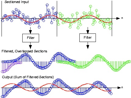


Consequently, we must literally add the filtered sections together, not just butt them together.
Figure 5.32.
The noisy input signal is sectioned into length-48 frames, each of which is filtered using frequency-domain techniques. Each filtered section is added to other outputs that overlap to create the signal equivalent to having filtered the entire input. The sinusoidal
component of the signal is shown as the red dashed line.
Computational considerations reveal a substantial advantage for a frequency-domain
implementation over a time-domain one. The number of computations for a time-domain
implementation essentially remains constant whether we section the input or not. Thus, the
number of computations for each output is
. In the frequency-domain approach, computation
counting changes because we need only compute the filter's frequency response H( k) once, which
amounts to a fixed overhead. We need only compute two DFTs and multiply them to filter a
section. Letting Nx denote a section's length, the number of computations for a section amounts to
( Nx+ q)log2( Nx+ q)+6( Nx+ q) . In addition, we must add the filtered outputs together; the number of terms to add corresponds to the excess duration of the output compared with the input ( q). The
frequency-domain approach thus requires
computations per output value.
For even modest filter orders, the frequency-domain approach is much faster.
Show that as the section length increases, the frequency domain approach becomes increasingly
more efficient.
Let N denote the input's total duration. The time-domain implementation requires a total of
N(2 q+1) computations, or 2 q+1 computations per input value. In the frequency domain, we split
the input into
sections, each of which requires
per input in the section.
Because we divide again by Nx to find the number of computations per input value in the entire

input, this quantity decreases as Nx increases. For the time-domain implementation, it stays
constant.
Note that the choice of section duration is arbitrary. Once the filter is chosen, we should section so
that the required FFT length is precisely a power of two: Choose Nx so that Nx+ q=2 L .
Implementing the digital filter shown in the A/D block diagram with a frequency-domain implementation requires some additional signal management not required by time-domain
implementations. Conceptually, a real-time, time-domain filter could accept each sample as it
becomes available, calculate the difference equation, and produce the output value, all in less that
the sampling interval Ts . Frequency-domain approaches don't operate on a sample-by-sample
basis; instead, they operate on sections. They filter in real time by producing Nx outputs for the
same number of inputs faster than NxTs . Because they generally take longer to produce an output
section than the sampling interval duration, we must filter one section while accepting into
memory the next section to be filtered. In programming, the operation of building up sections
while computing on previous ones is known as buffering. Buffering can also be used in time-
domain filters as well but isn't required.
Example 5.9.
We want to lowpass filter a signal that contains a sinusoid and a significant amount of noise.
The example shown in Figure 5.32 shows a portion of the noisy signal's waveform. If it
weren't for the overlaid sinusoid, discerning the sine wave in the signal is virtually impossible.
One of the primary applications of linear filters is noise removal: preserve the signal by
matching filter's passband with the signal's spectrum and greatly reduce all other frequency
components that may be present in the noisy signal.
A smart Rice engineer has selected a FIR filter having a unit-sample response corresponding a
period-17 sinusoid:
, n={0, …, 16} , which makes q=16 . Its frequency
response (determined by computing the discrete Fourier transform) is shown in Figure 5.33.
To apply, we can select the length of each section so that the frequency-domain filtering
approach is maximally efficient: Choose the section length Nx so that Nx+ q is a power of two.
To use a length-64 FFT, each section must be 48 samples long. Filtering with the difference
equation would require 33 computations per output while the frequency domain requires a
little over 16; this frequency-domain implementation is over twice as fast! Figure 5.32 shows
how frequency-domain filtering works.
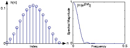

Figure 5.33.
The figure shows the unit-sample response of a length-17 Hanning filter on the left and the frequency response on the right. This
filter functions as a lowpass filter having a cutoff frequency of about 0.1.
We note that the noise has been dramatically reduced, with a sinusoid now clearly visible in
the filtered output. Some residual noise remains because noise components within the filter's
passband appear in the output as well as the signal.
Note that when compared to the input signal's sinusoidal component, the output's sinusoidal
component seems to be delayed. What is the source of this delay? Can it be removed?
The delay is not computational delay here--the plot shows the first output value is aligned with
the filter's first input--although in real systems this is an important consideration. Rather, the
delay is due to the filter's phase shift: A phase-shifted sinusoid is equivalent to a time-delayed
one:
. All filters have phase shifts. This delay could be removed if the
filter introduced no phase shift. Such filters do not exist in analog form, but digital ones can be
programmed, but not in real time. Doing so would require the output to emerge before the input
arrives!
5.8. Conclusions: Fast Fourier Transforms*
This book has developed a class of efficient algorithms based on index mapping and polynomial
algebra. This provides a framework from which the Cooley-Tukey FFT, the split-radix FFT, the
PFA, and WFTA can be derived. Even the programs implementing these algorithms can have a
similar structure. Winograd's theorems were presented and shown to be very powerful in both
deriving algorithms and in evaluating them. The simple radix-2 FFT provides a compact, elegant
means for efficiently calculating the DFT. If some elaboration is allowed, significant
improvement can be had from the split-radix FFT, the radix-4 FFT or the PFA. If multiplications
are expensive, the WFTA requires the least of all.
Several method for transforming real data were described that are more efficient than directly
using a complex FFT. A complex FFT can be used for real data by artificially creating a complex
input from two sections of real input. An alternative and slightly more efficient method is to
construct a special FFT that utilizes the symmetries at each stage.
As computers move to multiprocessors and multicore, writing and maintaining efficient programs
becomes more and more difficult. The highly structured form of FFTs allows automatic
generation of very efficient programs that are tailored specifically to a particular DSP or computer
architecture.
For high-speed convolution, the traditional use of the FFT or PFA with blocking is probably the
fastest method although rectangular transforms, distributed arithmetic, or number theoretic
transforms may have a future with special VLSI hardware.
The ideas presented in these notes can also be applied to the calculation of the discrete Hartley
transform 6, 2, the discrete cosine transform 3, 7, and to number theoretic transforms 1, 4, 5.
There are many areas for future research. The relationship of hardware to algorithms, the proper
use of multiple processors, the proper design and use of array processors and vector processors are
all open. There are still many unanswered questions in multi-dimensional algorithms where a
simple extension of one-dimensional methods will not suffice.
References
1. Blahut, Richard E. (1985). Fast Algorithms for Digital Signal Processing. Reading, Mass.:
Addison-Wesley.
2. Duhamel, P. and Vetterli, M. (1986, April). Cyclic Convolution of Real Sequences: Hartley
versus Fourier and New Schemes. Proceedings of the IEEE International Conference on
Acoustics, Speech, and Signal Processing (ICASSP-86), 6.5.
3. Elliott, D. F. and Rao, K. F. (1982). Fast Transforms: Algorithms, Analyses and Applications.
New York: Academic Press.
4. McClellan, J. H. and Rader, C. M. (1979). Number Theory in Digital Signal Processing.
Englewood Cliffs, NJ: Prentice-Hall.
5. Nussbaumer, H. J. (1981, 1982). Fast Fourier Transform and Convolution Algorithms.
(Second). Heidelberg, Germany: Springer-Verlag.
6. Sorensen, H. V. and Jones, D. L. and Burrus, C. S. and Heideman, M. T. (1985, October). On
Computing the Discrete Hartley Transform. IEEE Transactions on Acoustics, Speech, and
Signal Processing, 33(5), 1231–1238.


7. Vetterli, Martin and Nussbaumer, H. J. (1984, August). Simple FFT and DCT Algorithms with
Reduced Number of Operations. Signal Processing, 6(4), 267–278.
5.9. The Cooley-Tukey Fast Fourier Transform
Algorithm*
The publication by Cooley and Tukey 5 in 1965 of an efficient algorithm for the calculation of the
DFT was a major turning point in the development of digital signal processing. During the five or
so years that followed, various extensions and modifications were made to the original algorithm
4. By the early 1970's the practical programs were basically in the form used today. The standard
development presented in 21, 22, 2 shows how the DFT of a length-N sequence can be simply calculated from the two length-N/2 DFT's of the even index terms and the odd index terms. This is
then applied to the two half-length DFT's to give four quarter-length DFT's, and repeated until N
scalars are left which are the DFT values. Because of alternately taking the even and odd index
terms, two forms of the resulting programs are called decimation-in-time and decimation-in-
frequency. For a length of 2 M, the dividing process is repeated M=log2 N times and requires N
multiplications each time. This gives the famous formula for the computational complexity of the
FFT of N log2 N which was derived in Multidimensional Index Mapping: Equation 34.
Although the decimation methods are straightforward and easy to understand, they do not
generalize well. For that reason it will be assumed that the reader is familiar with that description
and this chapter will develop the FFT using the index map from Multidimensional Index
The Cooley-Tukey FFT always uses the Type 2 index map from Multidimensional Index
Mapping: Equation 11. This is necessary for the most popular forms that have N= RM, but is also used even when the factors are relatively prime and a Type 1 map could be used. The time and
frequency maps from Multidimensional Index Mapping: Equation 6 and Multidimensional
Index Mapping: Equation 12 are
(5.57)
(5.58)
Type-2 conditions Multidimensional Index Mapping: Equation 8 and Multidimensional Index
(5.59)


and
(5.60)
The row and column calculations in Multidimensional Index Mapping: Equation 15 are uncoupled by Multidimensional Index Mapping: Equation 16 which for this case are (5.61)
To make each short sum a DFT, the Ki must satisfy
(5.62)
In order to have the smallest values for Ki the constants in Equation 5.59 are chosen to be
(5.63)
a = d = K 2 = K 3 = 1
which makes the index maps of Equation 5.57 become
(5.64)
n = N 2 n 1 + n 2
(5.65)
k = k 1 + N 1 k 2
These index maps are all evaluated modulo N, but in Equation 5.64, explicit reduction is not
necessary since n never exceeds N. The reduction notation will be omitted for clarity. From
Multidimensional Index Mapping: Equation 15 and example Multidimensional Index
Mapping: Equation 19, the DFT is
(5.66)
This map of Equation 5.64 and the form of the DFT in Equation 5.66 are the fundamentals of the Cooley-Tukey FFT.
The order of the summations using the Type 2 map in Equation 5.66 cannot be reversed as it can
with the Type-1 map. This is because of the WN terms, the twiddle factors.
Turning Equation 5.66 into an efficient program requires some care. From Multidimensional
Index Mapping: Efficiencies Resulting from Index Mapping with the DFT we know that all the factors should be equal. If N= RM , with R called the radix, N 1 is first set equal to R and N 2 is then necessarily RM–1 . Consider n 1 to be the index along the rows and n 2 along the columns. T