256
2560
1540
1532
1528
5696
5186
5184
5184
4096 61440 45060 44924 44856 136704 128514 128480 128480
2
0
0
0
0
4
4
4
4
4
8
0
0
0
20
16
16
16
8
24
8
4
4
60
52
52
52
16
72
32
28
24
164
144
144
144
32
184
104
92
84
412
372
372
372
64
456
288
268
248
996
912
912
912
128
1080
744
700
660
2332
2164
2164
2164
256
2504
1824
1740
1656
5348
5008
5008
5008
512
5688
4328
4156
3988
12060
11380
11380
11380
1024 12744 10016 9676
9336
26852
25488
25488
25488
2048 28216 22760 22076 21396 59164
56436
56436
56436
4096 61896 50976 49612 48248 129252 123792 123792 123792
In Table 5.4 Mi and Ai refer to the number of real multiplications and real additions used by an
FFT with i separately written butterflies. The first block has the counts for Radix-2, the second for
Radix-4, the third for Radix-8, the fourth for Radix-16, and the last for the Split-Radix FFT. For
the split-radix FFT, M3 and A3 refer to the two- butterfly-plus program and M5 and A5 refer to
the three-butterfly program.
The first evaluations of FFT algorithms were in terms of the number of real multiplications
required as that was the slowest operation on the computer and, therefore, controlled the execution
speed. Later with hardware arithmetic both the number of multiplications and additions became
important. Modern systems have arithmetic speeds such that indexing and data transfer times
become important factors. Morris 19 has looked at some of these problems and has developed a
procedure called autogen to write partially straight-line program code to significantly reduce
overhead and speed up FFT run times. Some hardware, such as the TMS320 signal processing
chip, has the multiply and add operations combined. Some machines have vector instructions or
have parallel processors. Because the execution speed of an FFT depends not only on the
algorithm, but also on the hardware architecture and compiler, experiments must be run on the
system to be used.


In many cases the unscrambler or bit-reverse-counter requires 10% of the execution time,
therefore, if possible, it should be eliminated. In high-speed convolution where the convolution is
done by multiplication of DFT's, a decimation-in-frequency FFT can be combined with a
decimation-in-time inverse FFT to require no unscrambler. It is also possible for a radix-2 FFT to
do the unscrambling inside the FFT but the structure is not very regular 22, 14. Special structures can be found in 22 and programs for data that are real or have special symmetries are in 6, 8, 27.
Although there can be significant differences in the efficiencies of the various Cooley-Tukey and
Split-Radix FFTs, the number of multiplications and additions for all of them is on the order of
N log N. That is fundamental to the class of algorithms.
The Quick Fourier Transform, An FFT based on Symmetries
The development of fast algorithms usually consists of using special properties of the algorithm
of interest to remove redundant or unnecessary operations of a direct implementation. The
discrete Fourier transform (DFT) defined by
(5.72)
where
(5.73)
WN = e – j 2 π / N
has enormous capacity for improvement of its arithmetic efficiency. Most fast algorithms use the
periodic and symmetric properties of its basis functions. The classical Cooley-Tukey FFT and
prime factor FFT 1 exploit the periodic properties of the cosine and sine functions. Their use of
the periodicities to share and, therefore, reduce arithmetic operations depends on the factorability
of the length of the data to be transformed. For highly composite lengths, the number of floating-
point operation is of order
and for prime lengths it is of order N 2.
This section will look at an approach using the symmetric properties to remove redundancies. This
possibility has long been recognized 13, 16, 25, 20 but has not been developed in any systematic way in the open literature. We will develop an algorithm, called the quick Fourier transform
(QFT) 16, that will reduce the number of floating point operations necessary to compute the DFT
by a factor of two to four over direct methods or Goertzel's method for prime lengths. Indeed, it
seems the best general algorithm available for prime length DFTs. One can always do better by
using Winograd type algorithms but they must be individually designed for each length. The Chirp
Z-transform can be used for longer lengths.
Input and Output Symmetries
We use the fact that the cosine is an even function and the sine is an odd function. The kernel of


the DFT or the basis functions of the expansion is given by
(5.74)
which has an even real part and odd imaginary part. If the data x( n) are decomposed into their real
and imaginary parts and those into their even and odd parts, we have
(5.75)
where the even part of the real part of x( n) is given by
(5.76)
ue ( n ) = ( u ( n ) + u ( – n ) ) / 2
and the odd part of the real part is
(5.77)
uo ( n ) = ( u ( n ) – u ( – n ) ) / 2
with corresponding definitions of ve( n) and vo( n). Using Convolution Algorithms: Equation 32
with a simpler notation, the DFT of Convolution Algorithms: Equation 29 becomes
(5.78)
The sum over an integral number of periods of an odd function is zero and the sum of an even
function over half of the period is one half the sum over the whole period. This causes
Equation 5.72 and Equation 5.78 to become
(5.79)
for k=0,1,2,⋯, N–1.
The evaluation of the DFT using equation Equation 5.79 requires half as many real multiplication
and half as many real additions as evaluating it using Equation 5.72 or Equation 5.78. We have exploited the symmetries of the sine and cosine as functions of the time index n. This is
independent of whether the length is composite or not. Another view of this formulation is that we
have used the property of associatively of multiplication and addition. In other words, rather than
multiply two data points by the same value of a sine or cosine then add the results, one should add
the data points first then multiply the sum by the sine or cosine which requires one rather than two
multiplications.
Next we take advantage of the symmetries of the sine and cosine as functions of the frequency
index k. Using these symmetries on Equation 5.79 gives
(5.80)


(5.81)
for k=0,1,2,⋯, N/2–1. This again reduces the number of operations by a factor of two, this time
because it calculates two output values at a time. The first reduction by a factor of two is always
available. The second is possible only if both DFT values are needed. It is not available if you are
calculating only one DFT value. The above development has not dealt with the details that arise
with the difference between an even and an odd length. That is straightforward.
Further Reductions if the Length is Even
If the length of the sequence to be transformed is even, there are further symmetries that can be
exploited. There will be four data values that are all multiplied by plus or minus the same sine or
cosine value. This means a more complicated pre-addition process which is a generalization of the
simple calculation of the even and odd parts in Equation 5.76 and Equation 5.77 will reduce the size of the order N 2 part of the algorithm by still another factor of two or four. It the length is
divisible by 4, the process can be repeated. Indeed, it the length is a power of 2, one can show this
process is equivalent to calculating the DFT in terms of discrete cosine and sine transforms 10, 11
with a resulting arithmetic complexity of order
and with a structure that is well suited to
real data calculations and pruning.
If the flow-graph of the Cooley-Tukey FFT is compared to the flow-graph of the QFT, one notices
both similarities and differences. Both progress in stages as the length is continually divided by
two. The Cooley-Tukey algorithm uses the periodic properties of the sine and cosine to give the
familiar horizontal tree of butterflies. The parallel diagonal lines in this graph represent the
parallel stepping through the data in synchronism with the periodic basis functions. The QFT has
diagonal lines that connect the first data point with the last, then the second with the next to last,
and so on to give a “star" like picture. This is interesting in that one can look at the flow graph of
an algorithm developed by some completely different strategy and often find section with the
parallel structures and other parts with the star structure. These must be using some underlying
periodic and symmetric properties of the basis functions.
Arithmetic Complexity and Timings
A careful analysis of the QFT shows that 2 N additions are necessary to compute the even and odd
parts of the input data. This is followed by the length N/2 inner product that requires 4( N/2)2= N 2
real multiplications and an equal number of additions. This is followed by the calculations
necessary for the simultaneous calculations of the first half and last half of C( k) which requires
4( N/2)=2 N real additions. This means the total QFT algorithm requires M 2 real multiplications
and N 2+4 N real additions. These numbers along with those for the Goertzel algorithm 3, 1, 20 and the direct calculation of the DFT are included in the following table. Of the various order- N 2 DFT
algorithms, the QFT seems to be the most efficient general method for an arbitrary length N.


Table 5.5.
Algorithm
Real Mults. Real Adds Trig Eval.
Direct DFT
Mod. 2nd Order Goertzel N 2 + N
N
QFT
N 2
N 2 + 4 N
2 N
Timings of the algorithms on a PC in milliseconds are given in the following table.
Table 5.6.
Algorithm
N = 125 N = 256
Direct DFT
4.90
19.83
Mod. 2O. Goertzel 1.32
5.55
QFT
1.09
4.50
Chirp + FFT
1.70
3.52
These timings track the floating point operation counts fairly well.
Conclusions
The QFT is a straight-forward DFT algorithm that uses all of the possible symmetries of the DFT
basis function with no requirements on the length being composite. These ideas have been
proposed before, but have not been published or clearly developed by 16, 25, 24, 12. It seems that the basic QFT is practical and useful as a general algorithm for lengths up to a hundred or so.
Above that, the chirp z-transform 1 or other filter based methods will be superior. For special
cases and shorter lengths, methods based on Winograd's theories will always be superior.
Nevertheless, the QFT has a definite place in the array of DFT algorithms and is not well known.
A Fortran program is included in the appendix.
It is possible, but unlikely, that further arithmetic reduction could be achieved using the fact that
WN has unity magnitude as was done in second-order Goertzel algorithm. It is also possible that
some way of combining the Goertzel and QFT algorithm would have some advantages. A
development of a complete QFT decomposition of a DFT of length-2 M shows interesting structure
10, 11 and arithmetic complexity comparable to average Cooley-Tukey FFTs. It does seem better
suited to real data calculations with pruning.
References
1. Burrus, C. S. and Parks, T. W. (1985). DFT/FFT and Convolution Algorithms. New York: John
Wiley & Sons.
2. Brigham, E. Oran. (1988). The Fast Fourier Transform and Its Applications. [Expansion of the
1974 book]. Englewood Cliffs, NJ: Prentice-Hall.
3. Burrus, C. S. (1992). Goertzel's Algorithm. Unpublished Notes. ECE Dept., Rice University.
4. Cooley, James W. and Lewis, Peter A. W. and Welch, Peter D. (1967, June). Historical Notes
on the Fast Fourier Transform. IEEE Transactions on Audio and Electroacoustics, 15, 260–
262.
5. Cooley, J. W. and Tukey, J. W. (1965). An Algorithm for the Machine Calculation of Complex
Fourier Series. Math. Computat. , 19, 297–301.
6. DSP Committee, (Ed.). (1979). Digital Signal Processing II, selected reprints. New York:
IEEE Press.
7. Duhamel, P. and Hollmann, H. (1984, January 5). Split Radix FFT Algorithm. Electronic
Letters, 20(1), 14–16.
8. Duhamel, P. (1986, April). Implementation of `Split-Radix' FFT Algorithms for Complex,
Real, and Real-Symmetric Data. [A shorter version appeared in the ICASSP-85 Proceedings, p.
20.6, March 1985]. IEEE Trans. on ASSP, 34, 285–295.
9. Duhamel, P. and Vetterli, M. (1986, April). Cyclic Convolution of Real Sequences: Hartley
versus Fourier and New Schemes. Proceedings of the IEEE International Conference on
Acoustics, Speech, and Signal Processing (ICASSP-86), 6.5.
10. Guo, H. and Sitton, G. A. and Burrus, C. S. (1994, April 19–22). The Quick Discrete Fourier
Transform. In Proceedings of the IEEE International Conference on Acoustics, Speech, and
Signal Processing. (p. III:445–448). IEEE ICASSP-94, Adelaide, Australia
11. Guo, H. and Sitton, G. A. and Burrus, C. S. (1998, February). The Quick Fourier Transform: an
FFT based on Symmetries. IEEE Transactions on Signal Processing, 46(2), 335–341.
12. Heideman, M. T. (1985). private communication.
13. Heideman, M. T. and Johnson, D. H. and Burrus, C. S. (1985). Gauss and the History of the
FFT. Archive for History of Exact Sciences, 34(3), 265–277.
14. Johnson, H. W. and Burrus, C. S. (1984, March). An In-Order, In-Place Radix-2 FFT. In
Proceedings of the IEEE International Conference on Acoustics, Speech, and Signal
Processing. (p. 28A.2.1–4). San Diego, CA
15. Johnson, Steven G. and Frigo, Matteo. (2007, January). A Modified Split-Radix FFT with
Fewer Arithmetic Operations. IEEE Transactions on Signal Processing, 55(1), 111–119.
16. Kohne, John F. (1980, July). A Quick Fourier Transform Algorithm. (TR-1723). Technical
report. Naval Electronics Laboratory Center.
17. Markel, J. D. (1971, June). FFT Pruning. IEEE Trans on Audio and Electroacoustics, 19(4),
305–311.
18. Martens, J. B. (1984, August). Recursive Cyclotomic Factorization – A New Algorithm for
Calculating the Discrete Fourier Transform. IEEE Trans. on ASSP, 32(4), 750–762.
19. Morris, L. R. (1982, 1983). Digital Signal Processing Software. Toronto, Canada: DSPSW,
Inc.
20. Oppenheim, A. V. and Schafer, R. W. (1989). Discrete-Time Signal Processing. Englewood
Cliffs, NJ: Prentice-Hall.
21. Oppenheim, A. V. and Schafer, R. W. (1999). Discrete-Time Signal Processing. (Second).
[Earlier editions in 1975 and 1989]. Englewood Cliffs, NJ: Prentice-Hall.
22. Rabiner, L. R. and Gold, B. (1975). Theory and Application of Digital Signal Processing.
Englewood Cliffs, NJ: Prentice-Hall.
23. Sorensen, H. V. and Heideman, M. T. and Burrus, C. S. (1986, February). On Computing the
Split–Radix FFT. IEEE Transactions on Acoustics, Speech, and Signal Processing, 34(1), 152–
156.
24. Sitton, G. A. (1985). The QFT Algorithm.
25. Sitton, G. A. (1991, June). The QDFT: An Efficient Method for Short Prime Length DFTs.
26. Sorensen, H. V. and Jones, D. L. and Burrus, C. S. and Heideman, M. T. (1985, October). On
Computing the Discrete Hartley Transform. IEEE Transactions on Acoustics, Speech, and


Signal Processing, 33(5), 1231–1238.
27. Sorensen, H. V. and Jones, D. L. and Heideman, M. T. and Burrus, C. S. (1987, June). Real
Valued Fast Fourier Transform Algorithms. IEEE Transactions on Acoustics, Speech, and
Signal Processing, 35(6), 849–863.
28. Vetterli, Martin and Nussbaumer, H. J. (1984, August). Simple FFT and DCT Algorithms with
Reduced Number of Operations. Signal Processing, 6(4), 267–278.
29. Yavne, R. (1968). An Economical Method for Calculating the Discrete Fourier Transform. In
Fall Joint Computer Conference, AFIPS Conference Proceedings. (Vol. 33 part 1, p. 115–125).
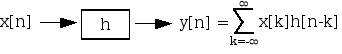
5.10. DTFT and Convolution*
Figure 5.38.
Given
X( ⅇⅈω) H( ⅇⅈω) Y( ⅇⅈω)
()
Let m= n− k→ n= m+ k
()
()
Y( ⅇⅈω)= X( ⅇⅈω) H( ⅇⅈω)
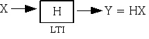

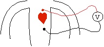
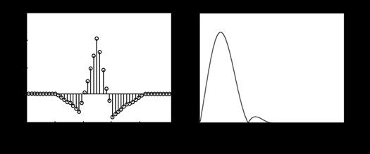
Figure 5.39.
()
Example 5.10. Lowpass Filtering of an ECG Signal to Suppress Noise
Figure 5.40.
ecg
voltages are very small ( μV !) therefore there is plenty of measurement noise
use DSP to reduce noise
simple processing: low pass filtering
Measurement process takes the TRUE SIGNAL
Figure 5.41.
and corrupts it with additive NOISE
Figure 5.42.
so that the actual received signal is SIGNAL+NOISE
Figure 5.43.
This is the signal we actually measure. It is "noisy".
Key Point
Signal is in low frequencies and noise is spread over all frequencies
We need a lowpass filter to suppress noise.
Try a simple averaging fil