4. The basic refinement equation (Equation) gives the scaling function in terms of a compressed
version of itself (self-similar). If we allow two (or more) scaling functions, each being a
weighted sum of a compress version of both, a more general set of basis functions results. This
can be viewed as a vector of scaling functions with the coefficients being a matrix now. Once
again, this generalization allows more flexibility in the characteristics of the individual
scaling functions and their related multi-wavelets. These are called multi-wavelet systems and
are still being developed.
5. One of the very few disadvantages of the discrete wavelet transform is the fact it is not shift
invariant. In other words, if you shift a signal in time, its wavelet transform not only shifts, it
changes character! For many applications in denoising and compression, this is not desirable
although it may be tolerable. The DWT can be made shift-invariant by calculating the DWT of
a signal for all possible shifts and adding (or averaging) the results. That turns out to be
equivalent to removing all of the down-samplers in the associated filter bank (an undecimated
filter bank), which is also equivalent to building an overdetermined or redundant DWT from a
traditional wavelet basis. This overcomplete system is similar to à`tight frame" and
maintains most of the features of an orthogonal basis yet is shift invariant. It does, however,
require N log ( N ) operations.
6. Wavelet systems are easily modified to being an adaptive system where the basis adjusts itself
to the properties of the signal or the signal class. This is often done by starting with a large
collection or library of expansion systems and bases. A subset is adaptively selected based on
the efficiency of the representation using a process sometimes called pursuit. In other words, a
set is chosen that will result in the smallest number of significant expansion coefficients.
Clearly, this is signal dependent, which is both its strength and its limitation. It is nonlinear.
7. One of the most powerful structures yet suggested for using wavelets for signal processing is
to first take the DWT, then do a point-wise linear or nonlinear processing of the DWT, finally
followed by an inverse DWT. Simply setting some of the wavelet domain expansion terms to
zero results in linear wavelet domain filtering, similar to what would happen if the same were
done with Fourier transforms. Donoho [link] [link] and others have shown by using some
form of nonlinear thresholding of the DWT, one can achieve near optimal denoising or
compression of a signal. The concentrating or localizing character of the DWT allows this
nonlinear thresholding to be very effective.
The present state of activity in wavelet research and application shows great promise based on the
above generalizations and extensions of the basic theory and structure [link]. We now have
conferences, workshops, articles, newsletters, books, and email groups that are moving the state of
the art forward. More details, examples, and software are given in [link] [link] [link].
References
1. C. Sidney Burrus, Ramesh A. Gopinath and Haitao Guo. (1998). Introduction to Wavelets and
the Wavelet Transform. Upper Saddle River, NJ: Prentice Hall.
2. Barbara Burke Hubbard. (1996). The World According to Wavelets. [Second Edition 1998].
Wellesley, MA: A K Peters.
3. C. Sidney Burrus. (1997, July). Wavelet Based Signal Processing: Where are We and Where
are We Going?, Plenary Talk. In Proceedings of the International Conference on Digital
Signal Processing. (Vol. I, pp. 3-5). Santorini, Greece
4. Ingrid Daubechies. (1992). Ten Lectures on Wavelets. [Notes from the 1990 CBMS-NSF
Conference on Wavelets and Applications at Lowell, MA]. Philadelphia, PA: SIAM.
5. Martin Vetterli and Jelena Kova\vcević. (1995). Wavelets and Subband Coding. Upper Saddle
River, NJ: Prentice-Hall.
6. Gilbert Strang and T. Nguyen. (1996). Wavelets and Filter Banks. Wellesley, MA: Wellesley-
Cambridge Press.
7. P. Steffen, P. N. Heller, R. A. Gopinath and C. S. Burrus. (1993, December). Theory of Regular
$M$-Band Wavelet Bases. [Special Transaction issue on wavelets; Rice contribution also in
Tech. Report No. CML TR-91-22, Nov. 1991.]. IEEE Transactions on Signal Processing,
41(12), 3497-3511.
8. Michel Misiti, Yves Misiti, Georges Oppenheim and Jean-Michel Poggi. (1996). Wavelet
Toolbox User's Guide. Natick, MA: The MathWorks, Inc.
Glossary
electrocardiogram
measure electrical signal given off by the heart.
Solutions
Chapter 6. ECE 454/ECE 554 Supplemental Reading for
Chapter 6
6.1. Discrete-Time Signals*
So far, we have treated what are known as analog signals and systems. Mathematically, analog
signals are functions having continuous quantities as their independent variables, such as space
and time. Discrete-time signals are functions defined on the integers; they are sequences. One of the fundamental results of signal theory will detail conditions under which an analog signal can be converted into a discrete-time one and retrieved without error. This result is important
because discrete-time signals can be manipulated by systems instantiated as computer programs.
Subsequent modules describe how virtually all analog signal processing can be performed with
software.
As important as such results are, discrete-time signals are more general, encompassing signals
derived from analog ones and signals that aren't. For example, the characters forming a text file
form a sequence, which is also a discrete-time signal. We must deal with such symbolic valued
signals and systems as well.
As with analog signals, we seek ways of decomposing real-valued discrete-time signals into
simpler components. With this approach leading to a better understanding of signal structure, we
can exploit that structure to represent information (create ways of representing information with
signals) and to extract information (retrieve the information thus represented). For symbolic-
valued signals, the approach is different: We develop a common representation of all symbolic-
valued signals so that we can embody the information they contain in a unified way. From an
information representation perspective, the most important issue becomes, for both real-valued
and symbolic-valued signals, efficiency; What is the most parsimonious and compact way to
represent information so that it can be extracted later.
Real- and Complex-valued Signals
A discrete-time signal is represented symbolically as s( n) , where n={ …, -1, 0, 1, …} . We usually draw discrete-time signals as stem plots to emphasize the fact they are functions defined only on
the integers. We can delay a discrete-time signal by an integer just as with analog ones. A delayed
unit sample has the expression δ( n− m) , and equals one when n= m .
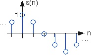


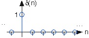
Figure 6.1. Discrete-Time Cosine Signal
The discrete-time cosine signal is plotted as a stem plot. Can you find the formula for this signal?
Complex Exponentials
The most important signal is, of course, the complex exponential sequence.
()
s( n)= ⅇⅈ 2 πfn
Sinusoids
Discrete-time sinusoids have the obvious form s( n)= A cos(2 πfn+ φ) . As opposed to analog
complex exponentials and sinusoids that can have their frequencies be any real value, frequencies
of their discrete-time counterparts yield unique waveforms only when f lies in the interval
.
This property can be easily understood by noting that adding an integer to the frequency of the
discrete-time complex exponential has no effect on the signal's value.
()
This derivation follows because the complex exponential evaluated at an integer multiple of
2 π equals one.
Unit Sample
The second-most important discrete-time signal is the unit sample, which is defined to be
()
Figure 6.2. Unit Sample
The unit sample.
Examination of a discrete-time signal's plot, like that of the cosine signal shown in Figure 6.1,

reveals that all signals consist of a sequence of delayed and scaled unit samples. Because the value
of a sequence at each integer m is denoted by s( m) and the unit sample delayed to occur at m is
written δ( n− m) , we can decompose any signal as a sum of unit samples delayed to the appropriate
location and scaled by the signal value.
()
This kind of decomposition is unique to discrete-time signals, and will prove useful subsequently.
Discrete-time systems can act on discrete-time signals in ways similar to those found in analog
signals and systems. Because of the role of software in discrete-time systems, many more
different systems can be envisioned and “constructed” with programs than can be with analog
signals. In fact, a special class of analog signals can be converted into discrete-time signals,
processed with software, and converted back into an analog signal, all without the incursion of
error. For such signals, systems can be easily produced in software, with equivalent analog
realizations difficult, if not impossible, to design.
Symbolic-valued Signals
Another interesting aspect of discrete-time signals is that their values do not need to be real
numbers. We do have real-valued discrete-time signals like the sinusoid, but we also have signals
that denote the sequence of characters typed on the keyboard. Such characters certainly aren't real
numbers, and as a collection of possible signal values, they have little mathematical structure
other than that they are members of a set. More formally, each element of the symbolic-valued
signal s( n) takes on one of the values { a 1, …, a K} which comprise the alphabet A . This technical terminology does not mean we restrict symbols to being members of the English or Greek
alphabet. They could represent keyboard characters, bytes (8-bit quantities), integers that convey
daily temperature. Whether controlled by software or not, discrete-time systems are ultimately
constructed from digital circuits, which consist entirely of analog circuit elements. Furthermore,
the transmission and reception of discrete-time signals, like e-mail, is accomplished with analog
signals and systems. Understanding how discrete-time and analog signals and systems intertwine
is perhaps the main goal of this course.
(This media type is not supported in this reader. Click to open media in browser.)
6.2. Difference Equation*


Introduction
One of the most important concepts of DSP is to be able to properly represent the input/output
relationship to a given LTI system. A linear constant-coefficient difference equation (LCCDE)
serves as a way to express just this relationship in a discrete-time system. Writing the sequence of
inputs and outputs, which represent the characteristics of the LTI system, as a difference equation
help in understanding and manipulating a system.
Definition: difference equation
An equation that shows the relationship between consecutive values of a sequence and the
differences among them. They are often rearranged as a recursive formula so that a systems
output can be computed from the input signal and past outputs.
Example .
()
y[ n]+7 y[ n−1]+2 y[ n−2]= x[ n]−4 x[ n−1]
General Formulas for the Difference Equation
As stated briefly in the definition above, a difference equation is a very useful tool in describing
and calculating the output of the system described by the formula for a given sample n. The key
property of the difference equation is its ability to help easily find the transform, H( z) , of a
system. In the following two subsections, we will look at the general form of the difference
equation and the general conversion to a z-transform directly from the difference equation.
Difference Equation
The general form of a linear, constant-coefficient difference equation (LCCDE), is shown below:
()
We can also write the general form to easily express a recursive output, which looks like this:
()
From this equation, note that y[ n− k] represents the outputs and x[ n− k] represents the inputs. The value of N represents the order of the difference equation and corresponds to the memory of the
system being represented. Because this equation relies on past values of the output, in order to
compute a numerical solution, certain past outputs, referred to as the initial conditions, must be


known.
Conversion to Z-Transform
Using the above formula, Equation, we can easily generalize the transfer function, H( z) , for any
difference equation. Below are the steps taken to convert any difference equation into its transfer
function, i.e. z-transform. The first step involves taking the Fourier Transform of all the terms in
Equation. Then we use the linearity property to pull the transform inside the summation and the
time-shifting property of the z-transform to change the time-shifting terms to exponentials. Once
this is done, we arrive at the following equation: a 0=1 .
Conversion to Frequency Response
Once the z-transform has been calculated from the difference equation, we can go one step further
to define the frequency response of the system, or filter, that is being represented by the difference
equation.
Remember that the reason we are dealing with these formulas is to be able to aid us in filter
design. A LCCDE is one of the easiest ways to represent FIR filters. By being able to find the
frequency response, we will be able to look at the basic properties of any filter represented by
a simple LCCDE.
Below is the general formula for the frequency response of a z-transform. The conversion is
simple a matter of taking the z-transform formula, H( z) , and replacing every instance of z with
ⅇⅈw .
Once you understand the derivation of this formula, look at the module concerning Filter Design


from the Z-Transform for a look into how all of these ideas of the Z-transform, Difference Equation, and Pole/Zero Plots play a role in filter design.
Example
Example 6.1. Finding Difference Equation
Below is a basic example showing the opposite of the steps above: given a transfer function
one can easily calculate the systems difference equation.
()
Given this transfer function of a time-domain filter, we want to find the difference equation.
To begin with, expand both polynomials and divide them by the highest order z.
()
From this transfer function, the coefficients of the two polynomials will be our ak and
bk values found in the general difference equation formula, Equation. Using these coefficients and the above form of the transfer function, we can easily write the difference equation:
()
In our final step, we can rewrite the difference equation in its more common form showing the
recursive nature of the system.
()
Solving a LCCDE
In order for a linear constant-coefficient difference equation to be useful in analyzing a LTI
system, we must be able to find the systems output based upon a known input, x( n) , and a set of
initial conditions. Two common methods exist for solving a LCCDE: the direct method and the
indirect method, the later being based on the z-transform. Below we will briefly discuss the
formulas for solving a LCCDE using each of these methods.
Direct Method


The final solution to the output based on the direct method is the sum of two parts, expressed in
the following equation:
()
y( n)= yh( n)+ yp( n)
The first part, yh( n) , is referred to as the homogeneous solution and the second part, yh( n) , is referred to as particular solution. The following method is very similar to that used to solve
many differential equations, so if you have taken a differential calculus course or used differential
equations before then this should seem very familiar.
Homogeneous Solution
We begin by assuming that the input is zero, x( n)=0 . Now we simply need to solve the
homogeneous difference equation:
()
In order to solve this, we will make the assumption that the solution is in the form of an
exponential. We will use lambda, λ, to represent our exponential terms. We now have to solve the
following equation:
()
We can expand this equation out and factor out all of the lambda terms. This will give us a large
polynomial in parenthesis, which is referred to as the characteristic polynomial. The roots of this
polynomial will be the key to solving the homogeneous equation. If there are all distinct roots,
then the general solution to the equation will be as follows:
()
yh( n)= C 1( λ 1) n+ C 2( λ 2) n+ …+ CN( λN) n
However, if the characteristic equation contains multiple roots then the above general solution
will be slightly different. Below we have the modified version for an equation where λ1 has K
multiple roots:
()
yh( n)= C 1( λ 1) n+ C 1 n( λ 1) n+ C 1 n 2( λ 1) n+ …+ C 1 nK−1( λ 1) n+ C 2( λ 2) n+ …+ CN( λN) n Particular Solution
The particular solution, yp( n) , will be any solution that will solve the general difference equation:


()
In order to solve, our guess for the solution to yp( n) will take on the form of the input, x( n) . After guessing at a solution to the above equation involving the particular solution, one only needs to
plug the solution into the difference equation and solve it out.
Indirect Method
The indirect method utilizes the relationship between the difference equation and z-transform,