

The final solution to the output based on the direct method is the sum of two parts, expressed in
the following equation:
()
y( t)= yh( t)+ yp( t)
The first part, yh( t) , is referred to as the homogeneous solution and the second part, yh( t) , is referred to as particular solution. The following method is very similar to that used to solve
many differential equations, so if you have taken a differential calculus course or used differential
equations before then this should seem very familiar.
Homogeneous Solution
We begin by assuming that the input is zero, x( t)=0 . Now we simply need to solve the
homogeneous differential equation:
()
In order to solve this, we will make the assumption that the solution is in the form of an
exponential. We will use lambda, λ, to represent our exponential terms. We now have to solve the
following equation:
()
We can expand this equation out and factor out all of the lambda terms. This will give us a large
polynomial in parenthesis, which is referred to as the characteristic polynomial. The roots of this
polynomial will be the key to solving the homogeneous equation. If there are all distinct roots,
then the general solution to the equation will be as follows:
()
yh( t)= C 1( λ 1) t+ C 2( λ 2) t+ …+ CN( λN) t
However, if the characteristic equation contains multiple roots then the above general solution
will be slightly different. Below we have the modified version for an equation where λ1 has K
multiple roots:
()
yh( t)= C 1( λ 1) t+ C 1 t( λ 1) t+ C 1 t 2( λ 1) t+ …+ C 1 tK−1( λ 1) t+ C 2( λ 2) t+ …+ CN( λN) t Particular Solution
The particular solution, yp( t) , will be any solution that will solve the general differential equation:


()
In order to solve, our guess for the solution to yp( t) will take on the form of the input, x( t) . After guessing at a solution to the above equation involving the particular solution, one only needs to
plug the solution into the differential equation and solve it out.
Indirect Method
The indirect method utilizes the relationship between the differential equation and the Laplace-
transform, discussed earlier, to find a solution. The basic idea is to convert the differential
equation into a Laplace-transform, as described above, to get the resulting output, Y( s) . Then by inverse transforming this and using partial-fraction expansion, we can arrive at the solution.
(6.14)
This can be interatively extended to an arbitrary order derivative as in Equation Equation 6.15.
(6.15)
Now, the Laplace transform of each side of the differential equation can be taken
(6.16)
which by linearity results in
(6.17)
and by differentiation properties in
(6.18)
Rearranging terms to isolate the Laplace transform of the output,
(6.19)
Thus, it is found that
(6.20)


In order to find the output, it only remains to find the Laplace transform X( s) of the input,
substitute the initial conditions, and compute the inverse Laplace transform of the result. Partial
fraction expansions are often required for this last step. This may sound daunting while looking at
Equation Equation 6.20, but it is often easy in practice, especially for low order differential
equations. Equation Equation 6.20 can also be used to determine the transfer function and
frequency response.
As an example, consider the differential equation
(6.21)
with the initial conditions y'(0)=1 and y(0)=0 Using the method described above, the Laplace
transform of the solution y( t) is given by
(6.22)
Performing a partial fraction decomposition, this also equals
(6.23)
Computing the inverse Laplace transform,
(6.24)
One can check that this satisfies that this satisfies both the differential equation and the initial
conditions.
Summary
One of the most important concepts of DSP is to be able to properly represent the input/output
relationship to a given LTI system. A linear constant-coefficient difference equation (LCCDE)
serves as a way to express just this relationship in a discrete-time system. Writing the sequence of
inputs and outputs, which represent the characteristics of the LTI system, as a difference equation
helps in understanding and manipulating a system.
Glossary
Definition: difference equation
An equation that shows the relationship between consecutive values of a sequence and the
differences among them. They are often rearranged as a recursive formula so that a systems
output can be computed from the input signal and past outputs. Example .
simplemath mathml-miitalicsy[ mathml-miitalicsn]+7 mathml-miitalicsy[ mathml-miitalicsn−1]+2
Definition: poles
1. The value(s) for simplemath mathml-miitalicsz z where Qz= .
2. The complex frequencies that make the overall gain of the filter transfer function infinite.
Definition: zeros
1. The value(s) for simplemath mathml-miitalicsz z where Pz= .
2. The complex frequencies that make the overall gain of the filter transfer function zero.
Solutions

Chapter 7. ECE 454/ECE 554 Supplemental Reading for
Chapter 7
7.1. Filtering in the Frequency Domain*
Because we are interested in actual computations rather than analytic calculations, we must
consider the details of the discrete Fourier transform. To compute the length- N DFT, we assume
that the signal has a duration less than or equal to N. Because frequency responses have an explicit
frequency-domain specification in terms of filter coefficients, we don't have a direct handle on which signal has a Fourier transform equaling a given frequency response. Finding this signal is
quite easy. First of all, note that the discrete-time Fourier transform of a unit sample equals one
for all frequencies. Because of the input and output of linear, shift-invariant systems are related to
each other by Y( ⅇⅈ 2 πf)= H( ⅇⅈ 2 πf) X( ⅇⅈ 2 πf) , a unit-sample input, which has X( ⅇⅈ2 πf)=1 , results in the output's Fourier transform equaling the system's transfer function.
This statement is a very important result. Derive it yourself.
The DTFT of the unit sample equals a constant (equaling 1). Thus, the Fourier transform of the
output equals the transfer function.
In the time-domain, the output for a unit-sample input is known as the system's unit-sample
response, and is denoted by h( n) . Combining the frequency-domain and time-domain
interpretations of a linear, shift-invariant system's unit-sample response, we have that h( n) and the
transfer function are Fourier transform pairs in terms of the discrete-time Fourier transform.
(7.1)
( h( n) ↔ H( ⅇⅈ 2 πf))
Returning to the issue of how to use the DFT to perform filtering, we can analytically specify the
frequency response, and derive the corresponding length- N DFT by sampling the frequency
response.
()
Computing the inverse DFT yields a length- N signal no matter what the actual duration of the
unit-sample response might be. If the unit-sample response has a duration less than or equal to N


(it's a FIR filter), computing the inverse DFT of the sampled frequency response indeed yields the
unit-sample response. If, however, the duration exceeds N, errors are encountered. The nature of
these errors is easily explained by appealing to the Sampling Theorem. By sampling in the
frequency domain, we have the potential for aliasing in the time domain (sampling in one domain,
be it time or frequency, can result in aliasing in the other) unless we sample fast enough. Here, the
duration of the unit-sample response determines the minimal sampling rate that prevents aliasing.
For FIR systems — they by definition have finite-duration unit sample responses — the number
of required DFT samples equals the unit-sample response's duration: N≥ q .
Derive the minimal DFT length for a length- q unit-sample response using the Sampling Theorem.
Because sampling in the frequency domain causes repetitions of the unit-sample response in the
time domain, sketch the time-domain result for various choices of the DFT length N.
In sampling a discrete-time signal's Fourier transform L times equally over [0, 2 π) to form the
DFT, the corresponding signal equals the periodic repetition of the original signal.
()
To avoid aliasing (in the time domain), the transform length must equal or exceed the signal's
duration.
Express the unit-sample response of a FIR filter in terms of difference equation coefficients. Note
that the corresponding question for IIR filters is far more difficult to answer: Consider the
The difference equation for an FIR filter has the form
()
The unit-sample response equals
()
which corresponds to the representation described in a problem of a length- q boxcar filter.
For IIR systems, we cannot use the DFT to find the system's unit-sample response: aliasing of the
unit-sample response will always occur. Consequently, we can only implement an IIR filter
accurately in the time domain with the system's difference equation. Frequency-domain
implementations are restricted to FIR filters.
Another issue arises in frequency-domain filtering that is related to time-domain aliasing, this
time when we consider the output. Assume we have an input signal having duration Nx that we
pass through a FIR filter having a length- q+1 unit-sample response. What is the duration of the
output signal? The difference equation for this filter is
()
y( n)= b 0 x( n)+ …+ bqx( n− q)
This equation says that the output depends on current and past input values, with the input value q
samples previous defining the extent of the filter's memory of past input values. For example, the
output at index Nx depends on x( Nx) (which equals zero), x( Nx−1) , through x( Nx− q) . Thus, the output returns to zero only after the last input value passes through the filter's memory. As the
input signal's last value occurs at index Nx−1 , the last nonzero output value occurs when
n− q= Nx−1 or n= q+ Nx−1 . Thus, the output signal's duration equals q+ Nx .
In words, we express this result as "The output's duration equals the input's duration plus the
filter's duration minus one.". Demonstrate the accuracy of this statement.
The unit-sample response's duration is q+1 and the signal's Nx . Thus the statement is correct.
The main theme of this result is that a filter's output extends longer than either its input or its unit-
sample response. Thus, to avoid aliasing when we use DFTs, the dominant factor is not the
duration of input or of the unit-sample response, but of the output. Thus, the number of values at
which we must evaluate the frequency response's DFT must be at least q+ Nx and we must
compute the same length DFT of the input. To accommodate a shorter signal than DFT length, we
simply zero-pad the input: Ensure that for indices extending beyond the signal's duration that the
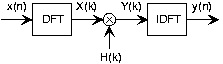
signal is zero. Frequency-domain filtering, diagrammed in Figure 7.1, is accomplished by storing
the filter's frequency response as the DFT H( k) , computing the input's DFT X( k) , multiplying
them to create the output's DFT Y( k)= H( k) X( k) , and computing the inverse DFT of the result to yield y( n) .
Figure 7.1.
To filter a signal in the frequency domain, first compute the DFT of the input, multiply the result by the sampled frequency response, and finally compute the inverse DFT of the product. The DFT's length must be at least the sum of the input's and unit-sample
response's duration minus one. We calculate these discrete Fourier transforms using the fast Fourier transform algorithm, of course.
Before detailing this procedure, let's clarify why so many new issues arose in trying to develop a
frequency-domain implementation of linear filtering. The frequency-domain relationship between


a filter's input and output is always true: Y( ⅇⅈ 2 πf)= H( ⅇⅈ 2 πf) X( ⅇⅈ 2 πf) . This Fourier transforms in this result are discrete-time Fourier transforms; for example,
. Unfortunately,
using this relationship to perform filtering is restricted to the situation when we have analytic
formulas for the frequency response and the input signal. The reason why we had to "invent" the
discrete Fourier transform (DFT) has the same origin: The spectrum resulting from the discrete-
time Fourier transform depends on the continuous frequency variable f. That's fine for analytic
calculation, but computationally we would have to make an uncountably infinite number of
computations.
Did you know that two kinds of infinities can be meaningfully defined? A countably infinite
quantity means that it can be associated with a limiting process associated with integers. An
uncountably infinite quantity cannot be so associated. The number of rational numbers is
countably infinite (the numerator and denominator correspond to locating the rational by row
and column; the total number so-located can be counted, voila!); the number of irrational
numbers is uncountably infinite. Guess which is "bigger?"
The DFT computes the Fourier transform at a finite set of frequencies — samples the true
spectrum — which can lead to aliasing in the time-domain unless we sample sufficiently fast. The
sampling interval here is for a length- K DFT: faster sampling to avoid aliasing thus requires a
longer transform calculation. Since the longest signal among the input, unit-sample response and
output is the output, it is that signal's duration that determines the transform length. We simply
extend the other two signals with zeros (zero-pad) to compute their DFTs.
Example 7.1.
Suppose we want to average daily stock prices taken over last year to yield a running weekly
average (average over five trading sessions). The filter we want is a length-5 averager (as
shown in the unit-sample response), and the input's duration is 253 (365 calendar days minus
weekend days and holidays). The output duration will be 253+5−1=257 , and this determines
the transform length we need to use. Because we want to use the FFT, we are restricted to
power-of-two transform lengths. We need to choose any FFT length that exceeds the required
DFT length. As it turns out, 256 is a power of two ( 28=256 ), and this length just undershoots
our required length. To use frequency domain techniques, we must use length-512 fast Fourier
transforms.
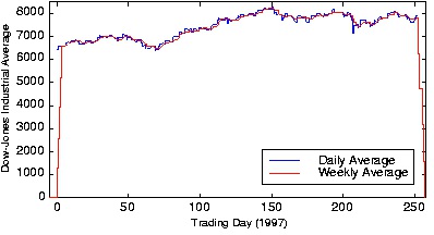
Figure 7.2.
The blue line shows the Dow Jones Industrial Average from 1997, and the red one the length-5 boxcar-filtered result that
provides a running weekly of this market index. Note the "edge" effects in the filtered output.
Figure 7.2 shows the input and the filtered output. The MATLAB programs that compute the
filtered output in the time and frequency domains are
Time Domain
h = [1 1 1 1 1]/5;
y = filter(h,1,[djia zeros(1,4)]);
Frequency Domain
h = [1 1 1 1 1]/5;
DJIA = fft(djia, 512);
H = fft(h, 512);
Y = H.*X;
y = ifft(Y);
The filter program has the feature that the length of its output equals the length of its
input. To force it to produce a signal having the proper length, the program zero-pads the
input appropriately.
MATLAB's fft function automatically zero-pads its input if the specified transform length
(its second argument) exceeds the signal's length. The frequency domain result will have a
small imaginary component — largest value is 2.2×10⁻¹¹ — because of the inherent finite
precision nature of computer arithmetic. Because of the unfortunate misfit between signal
lengths and favored FFT lengths, the number of arithmetic operations in the time-domain
implementation is far less than those required by the frequency domain version: 514 versus
62,271. If the input signal had been one sample shorter, the frequency-domain computations
would have been more than a factor of two less (28,696), but far more than in the time-domain
implementation.
An interesting signal processing aspect of this example is demonstrated at the beginning and


end of the output. The ramping up and down that occurs can be traced to assuming the input is
zero before it begins and after it ends. The filter "sees" these initial and final values as the
difference equation passes over the input. These artifacts can be handled in two ways: we can
just ignore the edge effects or the data from previous and succeeding years' last and first week,
respectively, can be placed at the ends.
7.2. FREQUENCY RESPONSE OF LTI (LSI)
SYSTEMS*
Up to now the discussion has been on discrete-time signals. As a matter of fact, most the
discussion so far also applies to systems (assumed to be LTI or LSI). However there are some
differences, e.g. the meaning of time convolution.
A system is characterized by its impulse h( n) whose DTFT transform is
()
And the inverse DTFT is
()
H( ω) is called the frequency response or frequency characteristic of the system. It is the frequency
characterization of the system whereas the impulse response is the time characterization.
Frequency response
Now we use the time convolution property (or convolution theorem) to map the output y( n) in
time domain to its transform Y( ω) in the frequency domain (Fig.3.28) :
()
y( n)= x( n)∗ h( n) ↔Y( ω)= X