Figure 7.13.
Example 7.8 (magnitude and phase spectra of the IIR notch filter)
Solution
The frequency response is
Figure 7.13shows the required spectra . The magnitude response gives a clear notes at frequency
ω=0.1π rad/sample
7.4. IIR Filtering: Introduction*
Introduction
Like finite impulse-response (FIR) filters, infinite impulse-response ( IIR) filters are linear
time-invariant ( LTI) systems that can recreate a large range of different frequency responses.
Compared to FIR filters, IIR filters have both advantages and disadvantages. On one hand,
implementing an IIR filter with certain stopband-attenuation and transition-band requirements
typically requires far fewer filter taps than an FIR filter meeting the same specifications. This
leads to a significant reduction in the computational complexity required to achieve a given
frequency response. However, the poles in the transfer function require feedback to implement an
IIR system. In addition to inducing nonlinear phase in the filter (delaying different frequency
input signals by different amounts), the feedback introduces complications in implementing IIR
filters on a fixed-point processor. Some of these complications are explored in IIR Filtering:
Filter-Coefficient Quanitization Exercise in MATLAB.
Later, in the processor exercise, you will explore the advantages and disadvantages of IIR filters
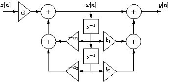
by implementing and examining a fourth-order IIR system on a fixed-point DSP. The IIR filter
should be implemented as a cascade of two second-order, Direct Form II sections. The data flow
for a second-order, Direct-Form II section, or bi-quad, is shown in Figure 7.14. Note that in
Direct Form II, the states (delayed samples) are neither the input nor the output samples, but are
instead the intermediate values w[ n] .
Figure 7.14.
Second-order, Direct Form II section
7.5. Discrete-Time Filtering Example*
Example 7.9.
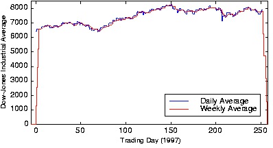
Suppose we want to average daily stock prices taken over last year to yield a running weekly
average (average over five trading sessions). The filter we want is a length-5 averager (as
shown in the unit-sample response), and the input's duration is 253 (365 calendar days minus weekend days and holidays). The output duration will be 253+5−1=257 , and this determines
the transform length we need to use. Because we want to use the FFT, we are restricted to
power-of-two transform lengths. We need to choose any FFT length that exceeds the required
DFT length. As it turns out, 256 is a power of two ( 28=256 ), and this length just undershoots
our required length. To use frequency domain techniques, we must use length-512 fast Fourier
transforms.
Figure 7.15.
The blue line shows the Dow Jones Industrial Average from 1997, and the red one the length-5 boxcar-filtered result that
provides a running weekly of this market index. Note the "edge" effects in the filtered output.
Figure 7.15 shows the input and the filtered output. The MATLAB programs that compute the
filtered output in the time and frequency domains are
Time Domain
h = [1 1 1 1 1]/5;
y = filter(h,1,[djia zeros(1,4)]);
Frequency Domain
h = [1 1 1 1 1]/5;
DJIA = fft(djia, 512);
H = fft(h, 512);
Y = H.*X;
y = ifft(Y);
The filter program has the "feature" that the length of its output equals the length of its
input. To force it to produce a signal having the proper length, the program zero-pads the
input appropriately.
MATLAB's fft function automatically zero-pads its input if the specified transform length
(its second argument) exceeds the signal's length. The frequency domain result will have a
small imaginary component — largest value is 2.2×10⁻¹¹ — because of the inherent finite
precision nature of computer arithmetic. Because of the unfortunate misfit between signal
lengths and favored FFT lengths, the number of arithmetic operations in the time-domain
implementation is far less than those required by the frequency domain version: 514 versus
62,271. If the input signal had been one sample shorter, the frequency-domain computations
would have been more than a factor of two less (28,696), but far more than in the time-domain
implementation.
An interesting signal processing aspect of this example is demonstrated at the beginning and
end of the output. The ramping up and down that occurs can be traced to assuming the input is
zero before it begins and after it ends. The filter "sees" these initial and final values as the
difference equation passes over the input. These artifacts can be handled in two ways: we can
just ignore the edge effects or the data from previous and succeeding years' last and first week,
respectively, can be placed at the ends.
7.6. FIR Filter Example*
Example 7.10.
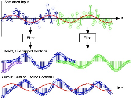
We want to lowpass filter a signal that contains a sinusoid and a significant amount of noise.
Figure 7.16 shows a portion of this signal's waveform. If it weren't for the overlaid sinusoid,
discerning the sine wave in the signal is virtually impossible. One of the primary applications
of linear filters is noise removal: preserve the signal by matching filter's passband with the
signal's spectrum and greatly reduce all other frequency components that may be present in
the noisy signal.
Figure 7.16.


The noisy input signal is sectioned into length-48 frames, each of which is filtered using frequency-domain techniques. Each
filtered section is added to other outputs that overlap to create the signal equivalent to having filtered the entire input. The
sinusoidal component of the signal is shown as the red dashed line.
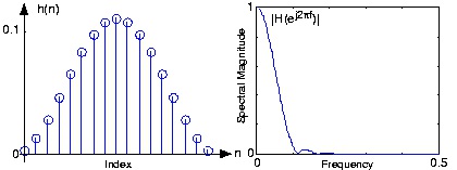
A smart Rice engineer has selected a FIR filter having a unit-sample response corresponding a
period-17 sinusoid:
, n∈{0, …, 16} , which makes q=16 . Its frequency
response (determined by computing the discrete Fourier transform) is shown in Figure 7.17.
To apply, we can select the length of each section so that the frequency-domain filtering
approach is maximally efficient: Choose the section length Nx so that Nx+ q is a power of two.
To use a length-64 FFT, each section must be 48 samples long. Filtering with the difference
equation would require 33 computations per output while the frequency domain requires a
little over 16; this frequency-domain implementation is over twice as fast! Figure 7.16 shows
how frequency-domain filtering works.
Figure 7.17.
The figure shows the unit-sample response of a length-17 Hanning filter on the left and the frequency response on the right. This
filter functions as a lowpass filter having a cutoff frequency of about 0.1.
We note that the noise has been dramatically reduced, with a sinusoid now clearly visible in
the filtered output. Some residual noise remains because noise components within the filter's
passband appear in the output as well as the signal.
Note that when compared to the input signal's sinusoidal component, the output's sinusoidal
component seems to be delayed. What is the source of this delay? Can it be removed?
The delay is not computational delay here—the plot shows the first output value is aligned with
the filter's first input—although in real systems this is an important consideration. Rather, the
delay is due to the filter's phase shift: A phase-shifted sinusoid is equivalent to a time-delayed
one:
. All filters have phase shifts. This delay could be removed if the filter
introduced no phase shift. Such filters do not exist in analog form, but digital ones can be
programmed, but not in real time. Doing so would require the output to emerge before the input
arrives!
7.7. Overview of Digital Filter Design*
Advantages of FIR filters
1. Straight forward conceptually and simple to implement
2. Can be implemented with fast convolution
3. Always stable
4. Relatively insensitive to quantization
5. Can have linear phase (same time delay of all frequencies)
Advantages of IIR filters
1. Better for approximating analog systems
2. For a given magnitude response specification, IIR filters often require much less computation
than an equivalent FIR, particularly for narrow transition bands
Both FIR and IIR filters are very important in applications.
Generic Filter Design Procedure
1. Choose a desired response, based on application requirements
2. Choose a filter class
3. Choose a quality measure
4. Solve for the filter in class 2 optimizing criterion in 3
Perspective on FIR filtering
Most of the time, people do L∞ optimal design, using the Parks-McClellan algorithm. This is probably the second most important technique in "classical" signal processing (after the Cooley-Tukey (radix-2) FFT).
Most of the time, FIR filters are designed to have linear phase. The most important advantage of
FIR filters over IIR filters is that they can have exactly linear phase. There are advanced design
techniques for minimum-phase filters, constrained L 2 optimal designs, etc. (see chapter 8 of text).


However, if only the magnitude of the response is important, IIR filers usually require much
fewer operations and are typically used, so the bulk of FIR filter design work has concentrated on
linear phase designs.
7.8. Window Design Method*
The truncate-and-delay design procedure is the simplest and most obvious FIR design procedure.
Is it any Good?
Yes; in fact it's optimal! (in a certain sense)
L2 optimization criterion
find h[ n] , 0≤ n≤ M−1 , maximizing the energy difference between the desired response and the
actual response: i.e., find
()
Since
this becomes
h[ n]
The best we can do is let
Thus h[ n]= hd[ n] w[ n] ,
is
optimal in a least-total-sqaured-error ( L 2 , or energy) sense!
Why, then, is this design often considered undersirable?
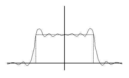
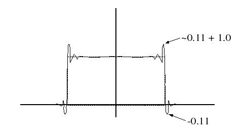

(b) A( ω) , large M
(a) A( ω) , small M
Figure 7.17.
For desired spectra with discontinuities, the least-square designs are poor in a minimax (worst-
case, or L∞ ) error sense.
Window Design Method
Apply a more gradual truncation to reduce "ringing" (Gibb's Phenomenon)
H( ω)= Hd( ω)* W( ω)
The window design procedure (except for the boxcar window) is ad-hoc and not optimal in any
usual sense. However, it is very simple, so it is sometimes used for "quick-and-dirty" designs of if
the error criterion is itself heurisitic.
7.9. Frequency Sampling Design Method for FIR filters*
Given a desired frequency response, the frequency sampling design method designs a filter with a
frequency response exactly equal to the desired response at a particular set of frequencies ωk .
(7.3)
Procedure


Desired Response must incluce linear phase shift (if linear phase is desired)
What is Hd( ω) for an ideal lowpass filter, cotoff at ωc ?
This set of linear equations can be written in matrix form
(7.4)
(7.5)
or
So
(7.6)
W N= M ωi≠ ωj+ 2πl i≠ j
Important Special Case
What if the frequencies are equally spaced between 0 and 2 π , i.e.
Then
so
or
Important Special Case #2


h[ n] symmetric, linear phase, and has real coefficients. Since h[ n]= h[ M− n] , there are only degrees of freedom, and only linear equations are required.
(7.7)
Removing linear phase from both sides yields
Due to
symmetry of response for real coefficients, only ωk on ω∈[0, π) need be specified, with the
frequencies – ωk thereby being implicitly defined also. Thus we have real-valued simultaneous
linear equations to solve for h[ n] .
Special Case 2a
h[ n] symmetric, odd length, linear phase, real coefficients, and ωk equally spaced:
(7.8)
To yield real coefficients, A( ω) mus be symmetric A( ω)= A(– ω)⇒ A[ k]= A[ M− k]


(7.9)
Simlar equations exist for even lengths, anti-symmetric, and
filter forms.
Comments on frequency-sampled design
This method is simple conceptually and very efficient for equally spaced samples, since h[ n] can
be computed using the IDFT.
H( ω) for a frequency sampled design goes exactly through the sample points, but it may be very
far off from the desired response for ω≠ ωk . This is the main problem with frequency sampled
design.
Possible solution to this problem: specify more frequency samples than degrees of freedom, and
minimize the total error in the frequency response at all of these samples.
Extended frequency sample design
For the samples H( ωk) where 0≤ k≤ M−1 and N> M , find h[ n] , where 0≤ n≤ M−1 minimizing
∥ Hd( ωk)− H( ωk)∥
For ∥ l∥∞ norm, this becomes a linear programming problem (standard packages availble!)
Here we will consider the ∥ l∥2 norm.
To minimize the ∥ l∥2 norm; that is,
, we have an overdetermined set of linear
equations:
or
The minimum error norm solution is well known to be
;
is well known as the
pseudo-inverse matrix.


Extended frequency sampled design discourages radical behavior of the frequency response
between samples for sufficiently closely spaced samples. However, the actual frequency
response may no longer pass exactly through any of the Hd( ωk) .
7.10. Parks-McClellan FIR Filter Design*
The approximation tolerances for a filter are very often given in terms of the maximum, or worst-
case, deviation within frequency bands. For example, we might wish a lowpass filter in a (16-bit)
CD player to have no more than -bit deviation in the pass and stop bands.
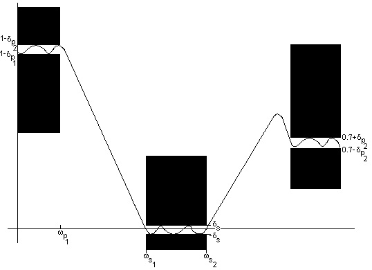
The Parks-McClellan filter design method efficiently designs linear-phase FIR filters that are
optimal in terms of worst-case (minimax) error. Typically, we would like to have the shortest-
length filter achieving these specifications. Figure Figure 7.18 illustrates the amplitude frequency
response of such a filter.

Figure 7.18.
The black boxes on the left and right are the passbands, the black boxes in the middle represent the stop band, and the space between the boxes are the transition bands. Note that overshoots may be allowed in the transition bands.
Must there be a transition band?
Yes, when the desired response is discontinuous. Since the frequency response of a finite-length
filter must be continuous, without a transition band the worst-case error could be no less than half
the discontinuity.
Formal Statement of the L-∞ (Minimax) Design Problem
For a given filter length ( M) and type (odd length, symmetric, linear phase, for example), and a
relative error weighting function W( ω) , find the filter coefficients minimizing the maximum
error
where E( ω)= W( ω)( Hd( ω)− H( ω)) and F is a compact subset of
ω∈[0, π] ( i.e. , all ω in the passbands and stop bands).
Typically, we would often rather specify ∥ E( ω)∥∞≤ δ and minimize over M and h; however,
the design techniques minimize δ for a given M. One then repeats the design procedure for
different M until the minimum M satisfying the requirements is found.
We will discuss in detail the design only of odd-length symmetric linear-phase FIR filters. Even-
length and anti-symmetric linear phase FIR filters are essentially the same except for a slightly
different implicit weighting function. For arbitrary phase, exactly optimal design procedures have
only recently been developed (1990).
Outline of L-∞ Filter Design
The Parks-McClellan method adopts an indirect method for finding the minimax-optimal filter
coefficients.
1. Using results from Approximation Theory, simple conditions for determining whether a given
filter is L∞ (minimax) optimal are found.
2. An iterative method for finding a filter which satisfies these conditions (and which is thus
optimal) is developed.


