A particular property of FIR filters that has proven to be very powerful is that a linear phase shift
for the frequency response is possible. This is especially important to time domain details of a
signal. The spectrum of a signal contains the individual frequency domain components separated
in frequency. The process of filtering usually involves passing some of these components and
rejecting others. This is done by multiplying the desired ones by one and the undesired ones by
zero. When they are recombined, it is important that the components have the same time domain
alignment as they originally did. That is exactly what linear phase insures. A phase response that
is linear with frequency keeps all of the frequency components properly registered with each
other. That is especially important in seismic, radar, and sonar signal analysis as well as for many
medical signals where the relative time locations of events contains the information of interest.
To develop the theory for linear phase FIR filters, a careful definition of phase shift is necessary.
If the real and imaginary parts of H( ω) are given by
(7.31)
where
and the magnitude is defined by
(7.32)
and the phase by
(7.33)
which gives
(7.34)
in terms of the magnitude and phase. Using the real and imaginary parts is using a rectangular
coordinate system and using the magnitude and phase is using a polar coordinate system. Often,


the polar system is easier to interpret.
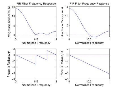
Mathematical problems arise from using | H( ω)| and Φ( ω), because | H( ω)| is not analytic and Φ( ω) not continuous. This problem is solved by introducing an amplitude function A( ω) that is real
valued and may be positive or negative. The frequency response is written as
(7.35)
where A( ω) is called the amplitude in order to distinguish it from the magnitude | H( ω)|, and Θ( ω) is the continuous version of Φ( ω). A( ω) is a real, analytic function that is related to the magnitude by
(7.36)
or
(7.37)
With this definition, A( ω) can be made analytic and Θ( ω) continuous. These are much easier to
work with than | H( ω)| and Φ( ω). The relationship of A( ω) and | H( ω)|, and of Θ( ω) and Φ( ω) are shown in Figure 7.24.
Figure 7.24.
Magnitude and Amplitude Frequency Responses and Corresponding Phase Frequency Response of Example Filter
To develop the characteristics and properties of linear-phase filters, assume a general linear plus
constant form for the phase function as
(7.38)
This gives the frequency response function of a length-N FIR filter as


(7.39)
and
(7.40)
Equation 7.40 can be put in the form of
(7.41)
if M (not necessarily an integer) is defined by
(7.42)
or equivalently,
(7.43)
Equation 7.40 then becomes
(7.44)
There are two possibilities for putting this in the form of Equation 7.41 where A( ω) is real: K 1=0
or K 1= π/2. The first case requires a special even symmetry in h( n) of the form
(7.45)
which gives
(7.46)
where A( ω) is the amplitude, a real-valued function of ω and e– jMω gives the linear phase with M
being the group delay. For the case where N is odd, using Equation 7.44, Equation 7.45, and
Equation 7.46, we have
(7.47)
or with a change of variables,
(7.48)


which becomes
(7.49)
where
is a shifted h( n). These formulas can be made simpler by defining new
coefficients so that Equation 7.47 becomes
(7.50)
where
(7.51)
and Equation 7.49 becomes
(7.52)
with
(7.53)
Notice from Equation 7.52 for N odd, A( ω) is an even function around ω=0 and ω= π, and is periodic with period 2 π.
For the case where N is even,
(7.54)
or with a change of variables,
(7.55)
These formulas can also be made simpler by defining new coefficients so that Equation 7.54
becomes
(7.56)
where


(7.57)
and Equation 7.55 becomes
(7.58)
with
(7.59)
Notice from Equation 7.58 for N even, A(ω) is an even function around ω=0, an odd function
around ω=π, and is periodic with period 4π. This requires A(π)=0.
For the case in Equation 7.41 where K 1= π/2, an odd symmetry is required of the form
(7.60)
which, for N odd, gives
(7.61)
with
(7.62)
and for N even
(7.63)
To calculate the frequency or amplitude response numerically, one must consider samples of the
continuous frequency response function above. L samples of the general complex frequency
response H( ω) in Equation 7.39 are calculated from
(7.64)
for k=0,1,2,⋯, L–1. This can be written with matrix notation as
(7.65)
where H is an L by 1 vector of the samples of the complex frequency response, F is the L by N
matrix of complex exponentials from Equation 7.64, and h is the N by 1 vector of real filter coefficients.


These equations are possibly redundant for equally spaced samples since A( ω) is an even function
and, if the phase response is linear, h( n) is symmetric. These redundancies are removed by
sampling Equation 7.50 over 0≤ ωk≤ π and by using a defined in Equation 7.51 rather than h. This can be written
(7.66)
where A is an L by 1 vector of the samples of the real valued amplitude frequency response, C is
the L by M real matrix of cosines from Equation 7.50, and a is the M by 1 vector of filter coefficients related to the impulse response by Equation 7.51. A similar set of equations can be
written from Equation 7.62 for N odd or from Equation 7.63 for N even.
This formulation becomes a filter design method by giving the samples of a desired amplitude
response as Ad( k) and solving Equation 7.66 for the filter coefficients a( n). If the number of independent frequency samples is equal to the number of independent filter coefficients and if C
is not singular, this is the frequency sampling filter design method and the frequency response of
the designed filter will interpolate the specified samples. If the number of frequency samples L is
larger than the number of filter coefficients N, Equation 7.66 may be solved approximately by
minimizing the norm ∥ A( ω)– Ad( ω)∥.
The Discrete Time Fourier Transform with Normalization
The discrete time Fourier transform of the impulse response of a digital filter is its frequency
response, therefore, it is an important tool. When the symmetry conditions of linear phase are
incorporated into the DTFT, it becomes similar to the discrete cosine or sine transform (DCT or
DST). It also has an arbitrary normalization possible for the odd length that needs to be
understood.
The discrete time Fourier transform (DTFT) is defined in Equation 7.25 which, with the
conditions of an odd length-N symmetrical signal, becomes
(7.67)
where M=( N–1)/2. Its inverse as
(7.68)
for n=1,2,⋯, M and
(7.69)
where K is a parameter of normalization for the a(0) term with 0< K<∞. If K=1, the expansion

equation Equation 7.67 is one summation and doesn't have to have the separate term for a(0). If K=1/2, the equation for the coefficients Equation 7.68 will also calculate the a(0) term and the separate equation Equation 7.69 is not needed. If
, a symmetry results which simplifies
equations later in the notes.
Four Types of Linear-Phase FIR Filters
From the previous discussion, it is seen that there are four possible types of FIR filters 1 that lead
to the linear phase of Equation 7.38. These are summarized in Table 7.1.
Table 7.1. The Four Types of Linear Phase FIR Filters
Type The impulse response has an odd length and is even symmetric about its midpoint of
1.
n= M=( N–1)/2 which requires h( n)= h( N– n–1) and gives Equation 7.47 and Equation 7.48.
The impulse response has an even length and is even symmetric about M, but M is not an
Type integer. Therefore, there is no h( n) at the point of symmetry, but it satisfies Equation 7.54
2.
and Equation 7.55.
The impulse response has an odd length as for Type 1 and has the odd symmetry of
Type Equation 7.60, giving an imaginary multiplier for the linear-phase form in Equation 7.61
3.
with amplitude Equation 7.62.
Type The impulse response has an even length as for Type 2 and the odd symmetry of Type 3 in
4.
Equation 7.60 and Equation 7.61 with amplitude Equation 7.63.
Examples of the four types of linear-phase FIR filters with the symmetries for odd and even
length are shown in Figure 7.25. Note that for N odd and h( n) odd symmetric, h( M)=0.
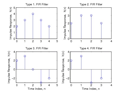
Figure 7.25.
Example of Impulse Responses for the Four Types of Linear Phase FIR Filters
For the analysis or design of linear-phase FIR filters, it is necessary to know the characteristics of
A( ω). The most important characteristics are shown in Table 7.2.
Table 7.2. Characteristics of A( ω) for Linear Phase
TYPE 1. Odd length, even symmetric h( n)
A( ω) is even about ω=0
A ( ω ) = A ( – ω )
A( ω) is even about ω= π
A ( π + ω ) = A ( π – ω )
A( ω) is periodic with period = 2 π A ( ω + 2 π ) = A ( ω )
TYPE 2. Even length, even symmetric h( n)
A( ω) is even about ω=0
A ( ω ) = A ( – ω )
A( ω) is odd about ω= π
A ( π + ω ) = – A ( π – ω )
A( ω) is periodic with period 4 π
A ( ω + 4 π ) = A ( ω )
TYPE 3. Odd length, odd symmetric h( n)
A( ω) is odd about ω=0
A ( ω ) = – A ( – ω )
A( ω) is odd about ω= π
A ( π + ω ) = – A ( π – ω )
A( ω) is periodic with period =2 π
A ( ω + 2 π ) = A ( ω )
TYPE 4. Even length, odd symmetric h( n)
A( ω) is odd about ω=0
A ( ω ) = – A ( – ω )
A( ω) is even about ω= π
A ( π + ω ) = A ( π – ω )
A( ω) is periodic with period =4 π
A ( ω + 4 π ) = A ( ω )
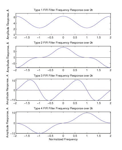
Examples of the amplitude function for odd and even length linear-phase filter A( ω) are shown in
Figure 7.26.
Example of Amplitude Responses for the Four Types of Linear Phase FIR Filters
These characteristics reveal several inherent features that are extremely important to filter design.
For Types 3 and 4, A(0)=0 for any choice of filter coefficients h( n). This would not be desirable
for a lowpass filter. Types 2 and 3 always have A( π)=0 which is not desirable for a highpass filter.
In addition to the linear-phase characteristic that represents a time shift, Types 3 and 4 give a
constant 90-degree phase shift, desirable for a differentiator or Hilbert transformer. The first step
in the design of a linear-phase FIR filter is the choice of the type most compatible with the


specifications.
It is possible to uses the formulas to express the frequency response of a general complex or non-
linear phase FIR filter by taking the even and odd parts of h( n) and calculating a real and
imaginary “amplitude" that would be added to give the actual frequency response.
Calculation of FIR Filter Frequency Response
As shown earlier, L equally spaced samples of H( ω) are easily calculated for L> N by appending L– N zeros to h( n) for a length-L DFT. This appears as
(7.70)
This direct method of calculation is a straightforward and flexible approach. Only the samples of
H( ω) that are of interest need to be calculated. In fact, even nonuniform spacing of the frequency
samples can be achieved by sampling the DTFT defined in Equation 7.25. The direct use of the
DFT can be inefficient, and for linear-phase filters, it is A( ω), not H( ω), that is the most
informative. In addition to the direct application of the DFT, special formulas are developed in
Equation 5 from FIR Filter Design by Frequency Sampling or Interpolation for evaluating samples of A( ω) that exploit the fact that h( n) is real and has certain symmetries. For long filters, even these formulas are too inefficient, so the DFT is used, but implemented by a Fast Fourier
Transform (FFT) algorithm.
In the special case of Type 1 filters with L equally spaced sample points, the samples of the
frequency response are of the form
(7.71)
For Type 2 filters,
(7.72)
For Type 3 filters,
(7.73)
For Type 4 filters,
(7.74)
Although this section has primarily concentrated on linear-phase filters by taking their

