2 N=16 additions for each stage and log2 N=3 stages, making the number of basic computations
as predicted.
FFT and the DFT
We now have a way of computing the spectrum for an arbitrary signal: The Discrete Fourier
Transform (DFT) computes the spectrum at N equally spaced frequencies from a length- N
sequence. An issue that never arises in analog "computation," like that performed by a circuit, is
how much work it takes to perform the signal processing operation such as filtering. In
computation, this consideration translates to the number of basic computational steps required to
perform the needed processing. The number of steps, known as the complexity, becomes
equivalent to how long the computation takes (how long must we wait for an answer). Complexity
is not so much tied to specific computers or programming languages but to how many steps are
required on any computer. Thus, a procedure's stated complexity says that the time taken will be
proportional to some function of the amount of data used in the computation and the amount
demanded.
For example, consider the formula for the discrete Fourier transform. For each frequency we
chose, we must multiply each signal value by a complex number and add together the results. For
a real-valued signal, each real-times-complex multiplication requires two real multiplications,
meaning we have 2 N multiplications to perform. To add the results together, we must keep the
real and imaginary parts separate. Adding N numbers requires N−1 additions. Consequently, each
frequency requires 2 N+2( N−1)=4 N−2 basic computational steps. As we have N frequencies, the
total number of computations is N(4 N−2) .
In complexity calculations, we only worry about what happens as the data lengths increase, and
take the dominant term—here the 4 N 2 term—as reflecting how much work is involved in making
the computation. As multiplicative constants don't matter since we are making a "proportional to"
evaluation, we find the DFT is an O( N 2) computational procedure. This notation is read "order N-
squared". Thus, if we double the length of the data, we would expect that the computation time to
approximately quadruple.
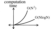
Speed Comparison
How much better is O(NlogN) than O( N 2 )?
Figure 9.11.
This figure shows how much slower the computation time of an O(NlogN) process grows.
Table 9.3.
N
10 100 1000
106
109
N 2
100 104
106
1012
1018
NlogN
1
200 3000 6×10⁶ 9×10⁹
Say you have a 1 MFLOP machine (a million "floating point" operations per second). Let
N=1million=106 .
An O( N 2 ) algorithm takes 1012 flors → 106 seconds ≃ 11.5 days.
An O( NlogN ) algorithm takes 6×10⁶ Flors → 6 seconds.
N=1million not
Example 9.3.
3 megapixel digital camera spits out 3×10⁶ numbers for each picture. So for two N point
sequences f[ n] and h[ n]. If computing ( f[ n] ⊛ h[ n]) directly: O( N 2 ) operations.
taking FFTs -- O(NlogN)
multiplying FFTs -- O(N)
inverse FFTs -- O(NlogN).
the total complexity is O(NlogN).
Conclusion
Other "fast" algorithms have been discovered, most of which make use of how many common
factors the transform length N has. In number theory, the number of prime factors a given integer
has measures how composite it is. The numbers 16 and 81 are highly composite (equaling 24 and
34 respectively), the number 18 is less so ( 2132 ), and 17 not at all (it's prime). In over thirty years
of Fourier transform algorithm development, the original Cooley-Tukey algorithm is far and away
the most frequently used. It is so computationally efficient that power-of-two transform lengths
are frequently used regardless of what the actual length of the data. It is even well established that


the FFT, alongside the digital computer, were almost completely responsible for the "explosion"
of DSP in the 60's.
9.3. The FFT Algorithm*
Definition: FFT
(Fast Fourier Transform) An efficient computational algorithm for computing the DFT.
The Fast Fourier Transform FFT
DFT can be expensive to compute directly
For each k, we must execute:
N complex multiplies
N−1 complex adds
The total cost of direct computation of an N-point DFT is
N 2 complex multiplies
N( N−1) complex adds
How many adds and mults of real numbers are required?
This " O( N 2) " computation rapidly gets out of hand, as N gets large:
Table 9.4.
N 1 10
100
1000 106
N 2 1 100 10,000 106
1012
Figure 9.12.


The FFT provides us with a much more efficient way of computing the DFT. The FFT requires
only " O( NlogN) " computations to compute the N-point DFT.
Table 9.5.
N
10
100
1000
106
N 2
100 10,000 106
1012
N log10 N 10
200
3000 6×10⁶
How long is 1012μsec ? More than 10 days! How long is 6×10⁶μsec ?
Figure 9.13.
The FFT and digital computers revolutionized DSP (1960 - 1980).
How does the FFT work?
The FFT exploits the symmetries of the complex exponentials
W kn
N are called " twiddle factors"
Symmetry
Symmetry
W kn
k( N+ n)
( k+ N) n
N = WN
= WN
Decimation in Time FFT
Just one of many different FFT algorithms
The idea is to build a DFT out of smaller and smaller DFTs by decomposing x[ n] into smaller
and smaller subsequences.


Assume N=2 m (a power of 2)
Derivation
N is even, so we can complete X[ k] by separating x[ n] into two subsequences each of length .
X[ k]=∑( x[ n] W kn
kn
N )+∑( x[ n] WN ) where
. So
()
where
. So
where
is -
point DFT of even samples ( G[ k] ) and
is -point DFT of odd samples ( H[ k] ).
X[ k]= G[ k]+ W k
N H[ k] , 0≤ k≤ N−1 Decomposition of an N-point DFT as a sum of 2
-point
DFTs.
Why would we want to do this? Because it is more efficient!
Recall
Cost to compute an N-point DFT is approximately N 2 complex mults and adds.
But decomposition into 2 -point DFTs + combination requires only
where
the first part is the number of complex mults and adds for -point DFT, G[ k] . The second part is
the number of complex mults and adds for -point DFT, H[ k] . The third part is the number of
complex mults and adds for combination. And the total is
complex mults and adds.
Example 9.4. Savings
For N=1000 , N 2=106
Because 1000 is small compared to 500,000,
So why stop here?! Keep decomposing. Break each of the -point DFTs into two -point DFTs,


etc. , ....
We can keep decomposing:
where m=log2 N= times
Computational cost: N -pt DFT two -pt DFTs. The cost is
. So replacing each -pt
DFT with two -pt DFTs will reduce cost to
As we keep
going p={3, 4, …, m} , where m=log2 N . We get the cost
N+ N log2 N is the total number of complex adds and mults.
For large N, cost≈ N log2 N or " O( N log2 N) ", since ( N log2 N ≫ N) for large N.
Figure 9.14.
N=8 point FFT. Summing nodes W k
n twiddle multiplication factors.
Weird order of time samples
Figure 9.15.
This is called "butterflies."
9.4. Overview of Fast Fourier Transform (FFT)
Algorithms*
A fast Fourier transform, or FFT, is not a new transform, but is a computationally efficient algorithm for the computing the DFT. The length- N DFT, defined as ()
where X( k) and x( n) are in general complex-valued and 0≤ k , n≤ N−1 , requires N complex multiplies to compute each X( k) . Direct computation of all N frequency samples thus requires

N 2 complex multiplies and N( N−1) complex additions. (This assumes precomputation of the DFT
coefficients
; otherwise, the cost is even higher.) For the large DFT lengths used in
many applications, N 2 operations may be prohibitive. (For example, digital terrestrial television
broadcast in Europe uses N = 2048 or 8192 OFDM channels, and the SETI project uses up to length-4194304 DFTs.) DFTs are thus almost always computed in practice by an FFT algorithm.
FFTs are very widely used in signal processing, for applications such as spectrum analysis and digital filtering via fast convolution.
History of the FFT
It is now known that C.F. Gauss invented an FFT in 1805 or so to assist the computation of planetary orbits via discrete Fourier series. Various FFT algorithms were independently invented over the next two centuries, but FFTs achieved widespread awareness and impact only with the
Cooley and Tukey algorithm published in 1965, which came at a time of increasing use of digital
computers and when the vast range of applications of numerical Fourier techniques was becoming
apparent. Cooley and Tukey's algorithm spawned a surge of research in FFTs and was also partly
responsible for the emergence of Digital Signal Processing (DSP) as a distinct, recognized
discipline. Since then, many different algorithms have been rediscovered or developed, and
efficient FFTs now exist for all DFT lengths.
Summary of FFT algorithms
The main strategy behind most FFT algorithms is to factor a length- N DFT into a number of
shorter-length DFTs, the outputs of which are reused multiple times (usually in additional short-
length DFTs!) to compute the final results. The lengths of the short DFTs correspond to integer
factors of the DFT length, N, leading to different algorithms for different lengths and factors. By
far the most commonly used FFTs select N=2 M to be a power of two, leading to the very efficient
power-of-two FFT algorithms, including the decimation-in-time radix-2 FFT and the
decimation-in-frequency radix-2 FFT algorithms, the radix-4 FFT ( N=4 M ), and the split-
radix FFT. Power-of-two algorithms gain their high efficiency from extensive reuse of
intermediate results and from the low complexity of length-2 and length-4 DFTs, which require no
multiplications. Algorithms for lengths with repeated common factors (such as 2 or 4 in the radix-2 and radix-4 algorithms, respectively) require extra twiddle factor multiplications between
the short-length DFTs, which together lead to a computational complexity of O( NlogN) , a very
considerable savings over direct computation of the DFT.
The other major class of algorithms is the Prime-Factor Algorithms (PFA). In PFAs, the short-length DFTs must be of relatively prime lengths. These algorithms gain efficiency by reuse of
intermediate computations and by eliminating twiddle-factor multiplies, but require more
operations than the power-of-two algorithms to compute the short DFTs of various prime lengths.


In the end, the computational costs of the prime-factor and the power-of-two algorithms are
comparable for similar lengths, as illustrated in Choosing the Best FFT Algorithm. Prime-length DFTs cannot be factored into shorter DFTs, but in different ways both Rader's conversion and the
chirp z-transform convert prime-length DFTs into convolutions of other lengths that can be computed efficiently using FFTs via fast convolution.
Some applications require only a few DFT frequency samples, in which case Goertzel's
algorithm halves the number of computations relative to the DFT sum. Other applications involve successive DFTs of overlapped blocks of samples, for which the running FFT can be more efficient than separate FFTs of each block.
9.5. Convolution Algorithms*
Fast Convolution by the FFT
One of the main applications of the FFT is to do convolution more efficiently than the direct
calculation from the definition which is:
(9.2)
which, with a change of variables, can also be written as:
(9.3)
This is often used to filter a signal x( n) with a filter whose impulse response is h( n). Each output value y( n) requires N multiplications and N–1 additions if y( n) and h( n) have N terms. So, for N
output values, on the order of N 2 arithmetic operations are required.
Because the DFT converts convolution to multiplication:
(9.4)
can be calculated with the FFT and bring the order of arithmetic operations down to N log( N)
which can be significant for large N.
This approach, which is called “fast convolutions", is a form of block processing since a whole
block or segment of x( n) must be available to calculate even one output value, y( n). So, a time
delay of one block length is always required. Another problem is the filtering use of convolution
is usually non-cyclic and the convolution implemented with the DFT is cyclic. This is dealt with
by appending zeros to x( n) and h( n) such that the output of the cyclic convolution gives one block
of the output of the desired non-cyclic convolution.
For filtering and some other applications, one wants “on going" convolution where the filter
response h( n) may be finite in length or duration, but the input x( n) is of arbitrary length. Two
methods have traditionally used to break the input into blocks and use the FFT to convolve the
block so that the output that would have been calculated by directly implementing Equation 9.2 or
Equation 9.3 can be constructed efficiently. These are called “overlap-add" and “over-lap save".
Fast Convolution by Overlap-Add
In order to use the FFT to convolve (or filter) a long input sequence x( n) with a finite length-M
impulse response, h( n), we partition the input sequence in segments or blocks of length L. Because
convolution (or filtering) is linear, the output is a linear sum of the result of convolving the first
block with h( n) plus the result of convolving the second block with h( n), plus the rest. Each of
these block convolutions can be calculated by using the FFT. The output is the inverse FFT of the
product of the FFT of x( n) and the FFT of h( n). Since the number of arithmetic operation to
calculate the convolution directly is on the order of M<