x[0]=4 x[1]=0 x[2]=0 x[3]=0
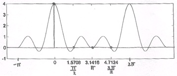
2. Sample DTFT. Using the same figure, Figure 3.34, we will take the DTFT of the signal and


get the following equations:
()
Our sample points will be:
where k={0, 1, 2, 3} (Figure 3.35).
Figure 3.35.
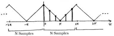
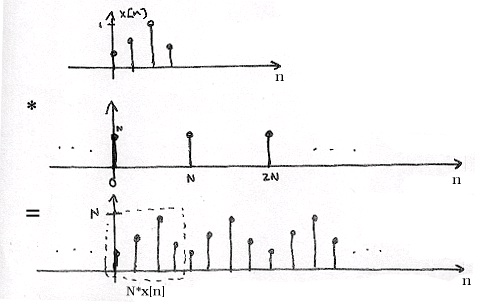
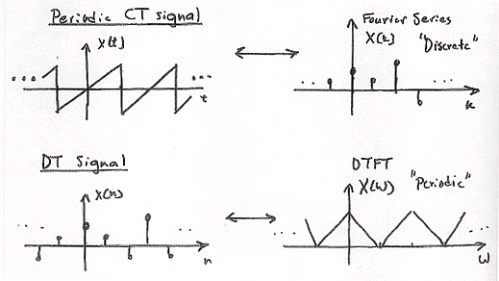
Periodicity of the DFT
DFT X[ k] consists of samples of DTFT, so X( ω) , a 2 π -periodic DTFT signal, can be converted to X[ k] , an N-periodic DFT.
()
where
is an N-periodic basis function (See Figure 3.36).
Figure 3.36.
Also, recall,

()
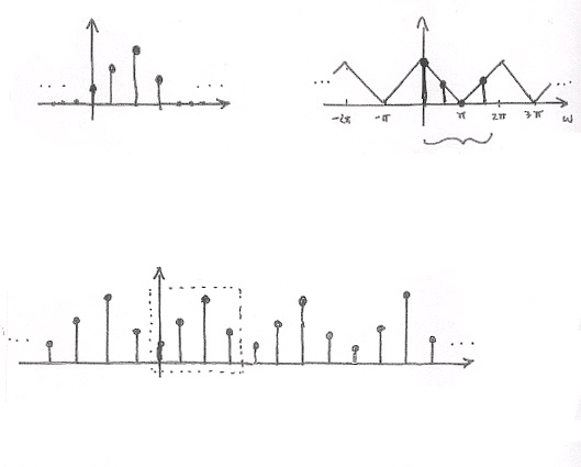
Example 3.14. Illustration
Figure 3.37.
When we deal with the DFT, we need to remember that, in effect, this treats the signal as
an N-periodic sequence.
A Sampling Perspective
Think of sampling the continuous function X( ω) , as depicted in Figure 3.38. S( ω) will represent the sampling function applied to X( ω) and is illustrated in Figure 3.38 as well. This will result in our discrete-time sequence, X[ k] .
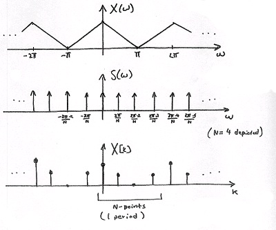


Figure 3.38.
Recall
Remember the multiplication in the frequency domain is equal to convolution in the time
domain!
Inverse DTFT of S(ω)
()
Given the above equation, we can take the DTFT and get the following equation:
()
Why does Equation equal S[ n] ?
S[ n] is N-periodic, so it has the following Fourier Series:
()


()
where the DTFT of the exponential in the above equation is equal to
.
So, in the time-domain we have (Figure 3.39):
Figure 3.39.
Connections
Figure 3.40.
Combine signals in Figure 3.40 to get signals in Figure 3.41.
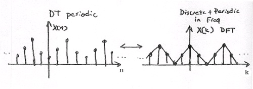

Figure 3.41.
3.14. Sampling Theorem*
Introduction
With the introduction of the concept of signal sampling, which produces a discrete time signal by
selecting the values of the continuous time signal at evenly spaced points in time, it is now
possible to discuss one of the most important results in signal processing, the Nyquist-Shannon
sampling theorem. Often simply called the sampling theorem, this theorem concerns signals,
known as bandlimited signals, with spectra that are zero for all frequencies with absolute value
greater than or equal to a certain level. The theorem implies that there is a sufficiently high
sampling rate at which a bandlimited signal can be recovered exactly from its samples, which is
an important step in the processing of continuous time signals using the tools of discrete time
signal processing.
Nyquist-Shannon Sampling Theorem
Statement of the Sampling Theorem
The Nyquist-Shannon sampling theorem concerns signals with continuous time Fourier transforms
that are only nonzero on the interval (– B, B) for some constant B. Such a function is said to be
bandlimited to (– B, B). Essentially, the sampling theorem has already been implicitly introduced in
the previous module concerning sampling. Given a continuous time signals x with continuous time
Fourier transform X, recall that the spectrum Xs of sampled signal xs with sampling period Ts is
given by
(3.25)


It had previously been noted that if x is bandlimited to
, the period of Xs centered
about the origin has the same form as X scaled in frequency since no aliasing occurs. This is
illustrated in Figure 3.42. Hence, if any two
bandlimited continuous time signals
sampled to the same signal, they would have the same continuous time Fourier transform and thus
be identical. Thus, for each discrete time signal there is a unique
bandlimited
continuous time signal that samples to the discrete time signal with sampling period Ts. Therefore,
this
bandlimited signal can be found from the samples by inverting this bijection.
This is the essence of the sampling theorem. More formally, the sampling theorem states the
following. If a signal x is bandlimited to (– B, B), it is completely determined by its samples with
sampling rate ωs=2 B. That is to say, x can be reconstructed exactly from its samples xs with
sampling rate ωs=2 B. The angular frequency 2 B is often called the angular Nyquist rate.
Equivalently, this can be stated in terms of the sampling period Ts=2 π/ ωs. If a signal x is
bandlimited to (– B, B), it is completely determined by its samples with sampling period Ts= π/ B.
That is to say, x can be reconstructed exactly from its samples xs with sampling period Ts.
Figure 3.42.
The spectrum of a bandlimited signals is shown as well as the spectra of its samples at rates above and below the Nyquist frequency.
As is shown, no aliasing occurs above the Nyquist frequency, and the period of the samples spectrum centered about the origin has the same form as the spectrum of the original signal scaled in frequency. Below the Nyquist frequency, aliasing can occur and causes the spectrum to take a different than the original spectrum.


Proof of the Sampling Theorem
The above discussion has already shown the sampling theorem in an informal and intuitive way
that could easily be refined into a formal proof. However, the original proof of the sampling
theorem, which will be given here, provides the interesting observation that the samples of a
signal with period Ts provide Fourier series coefficients for the original signal spectrum on
.
Let x be a
bandlimited signal and xs be its samples with sampling period Ts. We can
represent x in terms of its spectrum X using the inverse continuous time Fourier transfrom and the
fact that x is bandlimited. The result is
(3.26)
This representation of x may then be sampled with sampling period Ts to produce
(3.27)
Noticing that this indicates that xs( n) is the n th continuous time Fourier series coefficient for
X( ω) on the interval
, it is shown that the samples determine the original spectrum
X( ω) and, by extension, the original signal itself.
Perfect Reconstruction
Another way to show the sampling theorem is to derive the reconstruction formula that gives the
original signal
from its samples xs with sampling period Ts, provided x is bandlimited to
. This is done in the module on perfect reconstruction. However, the result, known as
the Whittaker-Shannon reconstruction formula, will be stated here. If the requisite conditions
hold, then the perfect reconstruction is given by
(3.28)
where the sinc function is defined as
(3.29)
From this, it is clear that the set
(3.30)
forms an orthogonal basis for the set of
bandlimited signals, where the coefficients of


a
signal in this basis are its samples with sampling period Ts.
Practical Implications
Discrete Time Processing of Continuous Time Signals
The Nyquist-Shannon Sampling Theorem and the Whittaker-Shannon Reconstruction formula
enable discrete time processing of continuous time signals. Because any linear time invariant
filter performs a multiplication in the frequency domain, the result of applying a linear time
invariant filter to a bandlimited signal is an output signal with the same bandlimit. Since sampling
a bandlimited continuous time signal above the Nyquist rate produces a discrete time signal with a
spectrum of the same form as the original spectrum, a discrete time filter could modify the
samples spectrum and perfectly reconstruct the output to produce the same result as a continuous
time filter. This allows the use of digital computing power and flexibility to be leveraged in
continuous time signal processing as well. This is more thouroughly described in the final module
of this chapter.
Psychoacoustics
The properties of human physiology and psychology often inform design choices in technologies
meant for interactin with people. For instance, digital devices dealing with sound use sampling
rates related to the frequency range of human vocalizations and the frequency range of human
auditory sensativity. Because most of the sounds in human speech concentrate most of their signal
energy between 5 Hz and 4 kHz, most telephone systems discard frequencies above 4 kHz and
sample at a rate of 8 kHz. Discarding the frequencies greater than or equal to 4 kHz through use of
an anti-aliasing filter is important to avoid aliasing, which would negatively impact the quality of
the output sound as is described in a later module. Similarly, human hearing is sensitive to
frequencies between 20 Hz and 20 kHz. Therefore, sampling rates for general audio waveforms
placed on CDs were chosen to be greater than 40 kHz, and all frequency content greater than or
equal to some level is discarded. The particular value that was chosen, 44.1 kHz, was selected for
other reasons, but the sampling theorem and the range of human hearing provided a lower bound
for the range of choices.
Sampling Theorem Summary
The Nyquist-Shannon Sampling Theorem states that a signal bandlimited to
can be
reconstructed exactly from its samples with sampling period Ts. The Whittaker-Shannon
interpolation formula, which will be further described in the section on perfect reconstruction,
provides the reconstruction of the unique
bandlimited continuous time signal that
samples to a given discrete time signal with sampling period Ts. This enables discrete time
processing of continuous time signals, which has many powerful applications.
Solutions
Chapter 4. ECE 454/ECE 554 Supplemental Reading for
Chapter 4
4.1. Examples for Systems in the Time Domain*
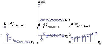
Example 4.1.
Let's consider the simple system having p=1 and q=0 .
()
y( n) ay( n−1)+ bx( n)
To compute the output at some index, this difference equation says we need to know what the
previous output y( n−1) and what the input signal is at that moment of time. In more detail,
let's compute this system's output to a unit-sample input: x( n)= δ( n) . Because the input is zero
for negative indices, we start by trying to compute the output at n=0 .
()
y(0)= ay(-1)+ b
What is the value of y(-1) ? Because we have used an input that is zero for all negative indices,
it is reasonable to assume that the output is also zero. Certainly, the difference equation would
not describe a linear system if the input that is zero for all time did not produce a zero output.
With this assumption, y(-1)=0 , leaving y(0)= b . For n>0 , the input unit-sample is zero,
which leaves us with the difference equation y( n)= ay( n−1) , n>0 . We can envision how the filter responds to this input by making a table.
()
y( n)= ay( n−1)+ bδ( n)
Table 4.1.
n x(n) y(n)
-1 0
0
0 b
b
1 0
ba
2 0
ba 2
:
0
:
n 0
ban
Coefficient values determine how the output behaves. The parameter b can be any value, and
serves as a gain. The effect of the parameter a is more complicated (Table 4.1). If it equals
zero, the output simply equals the input times the gain b. For all non-zero values of a, the
output lasts forever; such systems are said to be IIR ( Infinite Impulse Response). The reason
for this terminology is that the unit sample also known as the impulse (especially in analog
situations), and the system's response to the "impulse" lasts forever. If a is positive and less
than one, the output is a decaying exponential. When a=1, the output is a unit step. If a is
negative and greater than –1, the output oscillates while decaying exponentially. When a=1 ,
the output changes sign forever, alternating between b and – b. More dramatic effects when
| a|>1 ; whether positive or negative, the output signal becomes larger and larger, growing
exponentially.
Figure 4.1.
The input to the simple example system, a unit sample, is shown at the top, with the outputs for several system parameter values
shown below.
Positive values of a are used in population models to describe how population size increases
over time. Here, n might correspond to generation. The difference equation says that the
number in the next generation is some multiple of the previous one. If this multiple is less
than one, the population becomes extinct; if greater than one, the population flourishes. The
same difference equation also describes the effect of compound interest on deposits. Here, n
indexes the times at which compounding occurs (daily, monthly, etc. ), a equals the compound
interest rate plus one, and b=1 (the bank provides no gain). In signal processing applications,
we typically require that the output remain bounded for any input. For our example, that
means that we restrict | a|=1 and chose values for it and the gain according to the application.
Note that the difference equation,
(4.1)
the difference equation


y( n)= a 1 y( n−1)+ …+ apy( n− p)+ b 0 x( n)+ b 1 x( n−1)+ …+ bqx( n− q) does not involve terms like y( n+1) or x( n+1) on the equation's right side. Can such terms also be
included? Why or why not?
Such terms would require the system to know what future input or output values would be before
the current value was computed. Thus, such terms can cause difficulties.
Figure 4.2.
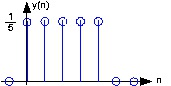
The plot shows the unit-sample response of a length-5 boxcar filter.
Example 4.2.
A somewhat different system has no "a" coefficients. Consider the difference equation
()
Because this system's output depends only on current and previous input values, we need not
be concerned with initial conditions. When the input is a unit-sample, the output equals for
n=[0, …, q−1] , then equals zero thereafter. Such systems are said to be FIR (Finite Impulse
Response) because their unit sample responses have finite duration. Plotting this response
(Figure 4.2) shows that the unit-sample response is a pulse of width q and height . This
waveform is also known as a boxcar, hence the name boxcar filter given to this system.
(We'll derive its frequency response and develop its filtering interpretation in the next
section.) For now, note that the difference equation says that each output value equals the
average of the input's current and previous values. Thus, the output equals the running
average of input's previous q values. Such a system could be used to produce the average
weekly temperature ( q=7 ) that could be updated daily.
4.2. Discrete-Time Processing of CT Signals*
DT Processing of CT Signals
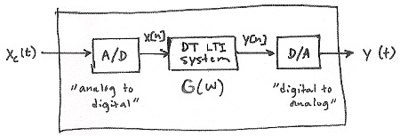


Figure 4.3. DSP System
Analysis
()
Yc( Ω)= H LP( Ω) Y( ΩT)
where we know that Y( ω)= X( ω) G( ω) and G( ω) is the frequency response of the DT LTI system.
Also, remember that ω≡ ΩT So,
()
Yc( Ω)= H LP( Ω) G( ΩT)