the end of the non-cyclic output of y ( n ) to the values at the beginning. This is a natural part of
cyclic convolution but is destructive if non-cyclic convolution is desired and is called aliasing or
folding for obvious reasons. Aliasing is a phenomenon that occurs in several arenas of DSP and
the matrix formulation makes it easy to understand.
References
1. Thomas F. Coleman and Charles Van Loan. (1988). Handbook for Matrix Computation.
Philadelphia, PA: SIAM.
Glossary
Definition: linear shift invariant system
A linear shift invariant system is one that is both:
linear
shift invariant
Solutions


Chapter 5. ECE 454/ECE 554 Supplemental Reading for
Chapter 5
5.1. DFT as a Matrix Operation*
Matrix Review
Recall:
Vectors in ℝ N :
Vectors in ℂ N :
Transposition:
1. transpose:
2. conjugate:
1. real:
2. complex:
Matrix Multiplication:
Matrix Transposition:
Matrix transposition involved simply
swapping the rows with columns.
The above equation is Hermitian transpose.
[AT] kn=A nk


Representing DFT as Matrix Operation
Now let's represent the DFT in vector-matrix notation.
Here x is the
vector of time samples and X is the vector of DFT coefficients. How are x and X related:
where
so X= Wx where X is the DFT vector, W is the matrix
and x the time domain vector.
IDFT:
where
is the matrix Hermitian transpose. So,
where x is the time vector,
is the inverse DFT matrix, and X is the DFT vector.
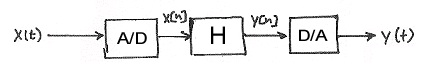
5.2. Filtering with the DFT*
Introduction
Figure 5.1.
()
()
Y( ω)= X( ω) H( ω)
Assume that H( ω) is specified.
How can we implement X( ω) H( ω) in a computer?
Discretize (sample) X( ω) and H( ω) . In order to do this, we should take the DFTs of x[ n] and h[ n] to get X[ k] and X[ k] . Then we will compute
Does
?
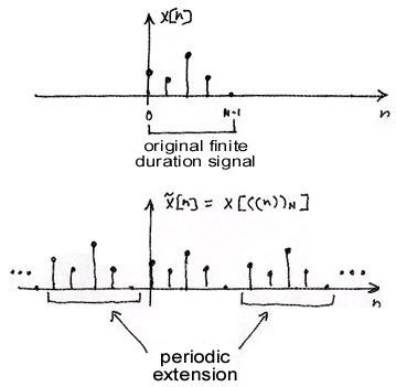


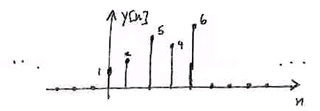
Recall that the DFT treats N-point sequences as if they are periodically extended (Figure 5.2): Figure 5.2.
Compute IDFT of Y[k]
()
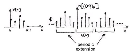
And the IDFT periodically extends h[ n] :
This computes as shown in Figure 5.3:
Figure 5.3.

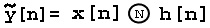


()
is called circular convolution and is denoted by Figure 5.4.
Figure 5.4.
The above symbol for the circular convolution is for an N-periodic extension.
DFT Pair
Figure 5.5.
Note that in general:
Figure 5.6.
Example 5.1. Regular vs. Circular Convolution
To begin with, we are given the following two length-3 signals:
x[ n]={1, 2, 3} h[ n]={1, 0, 2} We can zero-pad these signals so that we have the following
discrete sequences: x[ n]={ …, 0, 1, 2, 3, 0, …} h[ n]={ …, 0, 1, 0, 2, 0, …} where x[0]=1 and h[0]=1 .
Regular Convolution:
()
Using the above convolution formula (refer to the link if you need a review of
convolution), we can calculate the resulting value for y[0] to y[4] . Recall that because we have two length-3 signals, our convolved signal will be length-5.
n=0 { …, 0, 0, 0, 1, 2, 3, 0, …} { …, 0, 2, 0, 1, 0, 0, 0, …}
()
n=1 { …, 0, 0, 1, 2, 3, 0, …} { …, 0, 2, 0, 1, 0, 0, …}
()


n=2 { …, 0, 1, 2, 3, 0, …} { …, 0, 2, 0, 1, 0, …}
()
n=3
()
y[3]=4
n=4
()
y[4]=6
Figure 5.7. Regular Convolution Result
Result is finite duration, not periodic!
Circular Convolution:
()
And now with circular convolution our h[ n] changes and becomes a periodically extended
signal:
()
h[ (( n )) N]={ …, 1, 0, 2, 1, 0, 2, 1, 0, 2, …}
n=0 { …, 0, 0, 0, 1, 2, 3, 0, …} { …, 1, 2, 0, 1, 2, 0, 1, …}
()
n=1 { …, 0, 0, 0, 1, 2, 3, 0, …} { …, 0, 1, 2, 0, 1, 2, 0, …}
()
n=2
()
n=3
()
n=4
()
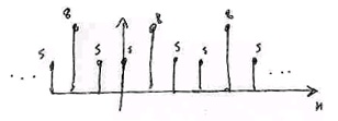
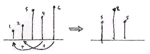


Figure 5.8. Circular Convolution Result
Result is 3-periodic.
Figure 5.9 illustrates the relationship between circular convolution and regular convolution
using the previous two figures:
Figure 5.9. Circular Convolution from Regular
The left plot (the circular convolution results) has a "wrap-around" effect due to periodic extension.
Regular Convolution from Periodic Convolution
1. "Zero-pad" x[ n] and h[ n] to avoid the overlap (wrap-around) effect. We will zero-pad the two signals to a length-5 signal (5 being the duration of the regular convolution result):
x[ n]={1, 2, 3, 0, 0} h[ n]={1, 0, 2, 0, 0}
2. Now take the DFTs of the zero-padded signals:
()
Now we can plot this result (Figure 5.10):
Figure 5.10.
The sequence from 0 to 4 (the underlined part of the sequence) is the regular convolution result. From this illustration we can see that it is 5-periodic!
General Result
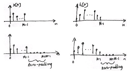


We can compute the regular convolution result of a convolution of an M-point signal x[ n] with
an N-point signal h[ n] by padding each signal with zeros to obtain two M+ N−1 length
sequences and computing the circular convolution (or equivalently computing the IDFT of
H[ k] X[ k] , the product of the DFTs of the zero-padded signals) (Figure 5.11).
Figure 5.11.
Note that the lower two images are simply the top images that have been zero-padded.
DSP System
Figure 5.12.
The system has a length N impulse response, h[ n]
1. Sample finite duration continuous-time input x( t) to get x[ n] where n={0, …, M−1} .
2. Zero-pad x[ n] and h[ n] to length M+ N−1 .
3. Compute DFTs X[ k] and H[ k]
4. Compute IDFTs of X[ k] H[ k]
where n={0, …, M+ N−1} .
5. Reconstruct y( t)
5.3. m10 - The Discrete Fourier Transform*


The Discrete Fourier Transform
The description of signals in terms of their sinusoidal frequency content has proven to be as
powerful and informative for discrete-time signals as it has for continuous-time signals. It is also
probably the most powerful computational tool we will use. We now develop the basic discrete-
time methods starting with the discrete Fourier transform (DFT) applied to finite length signals,
followed by the discrete-time Fourier transform (DTFT) for infinitely long signals, and ending
with the z-transform which uses the powerful tools of complex variable theory.
Definition of the DFT
It is assumed that the signal x ( n ) to be analyzed is a sequence of N real or complex values which
are a function of the integer variable n . The DFT of x ( n ) , also called the spectrum of x ( n ) , is a length N sequence of complex numbers denoted C ( k ) and defined by
()
using the usual engineering notation:
. The inverse transform (IDFT) which retrieves
x ( n ) from C ( k ) is given by
()
which is easily verified by substitution into (1). Indeed, this verification will require using the
orthogonality of the basis function of the DFT which is
()
The exponential basis functions,
, for k ∈ { 0 , N − 1 } , are the N values of the N th roots of
unity (the N zeros of the polynomial ( s − 1 ) N ). This property is what connects the DFT to
convolution and allows efficient algorithms for calculation to be developed [link]. They are used so often that the following notation is defined by
()
with the subscript being omitted if the sequence length is obvious from context. Using this
notation, the DFT becomes
()
One should notice that with the finite summation of the DFT, there is no question of convergence


or of the ability to interchange the order of summation. Nò`delta functions' are needed and the
N transform values can be calculated exactly (within the accuracy of the computer or calculator
used) from the N signal values with a finite number of arithmetic operations.
Matrix Formulation of the DFT
There are several advantages to using a matrix formulation of the DFT. This is given by writing
(Equation) or (Equation) in matrix operator form as
()
or
()
The orthogonality of the basis function in (Equation) shows up in this matrix formulation by the
columns of F being orthogonal to each other as are the rows. This means that
, where k is a
scalar constant, and, therefore,
. This is called a unitary operator.
The definition of the DFT in (Equation) emphasizes the fact that each of the N DFT values are the sum of N products. The matrix formulation in (Equation) has two interpretations. Each k -th DFT
term is the inner product of two vectors, k -th row of and ; or, the DFT vector, is a weighted
sum of the N columns of with weights being the elements of the signal vector . A third view of
the DFT is the operator view which is simply the single matrix equation (Equation).
It is instructive at this point to write a computer program to calculate the DFT of a signal. In
Matlab [link], there is a pre-programmed function to calculate the DFT, but that hides the scalar operations. One should program the transform in the scalar interpretive language of Matlab or
some other lower level language such as FORTRAN, C, BASIC, Pascal, etc. This will illustrate
how many multiplications and additions and trigonometric evaluations are required and how much
memory is needed. Do not use a complex data type which also hides arithmetic, but use Euler's
relations
()
ejx = cos ( x ) + j sin ( x )
to explicitly calculate the real and imaginary part of C ( k ) .
If Matlab is available, first program the DFT using only scalar operations. It will require two
nested loops and will run rather slowly because the execution of loops is interpreted. Next,
program it using vector inner products to calculate each C ( k ) which will require only one loop
and will run faster. Finally, program it using a single matrix multiplication requiring no loops and

running much faster. Check the memory requirements of the three approaches.
The DFT and IDFT are a completely well-defined, legitimate transform pair with a sound
theoretical basis that do not need to be derived from or interpreted as an approximation to the
continuous-time Fourier series or integral. The discrete-time and continuous-time transforms and
other tools are related and have parallel properties, but neither depends on the other.
The notation used here is consistent with most of the literature and with the standards given in
[link]. The independent index variable n of the signal x ( n ) is an integer, but it is usually interpreted as time or, occasionally, as distance. The independent index variable k of the DFT
C ( k ) is also an integer, but it is generally considered as frequency. The DFT is called the
spectrum of the signal and the magnitude of the complex valued DFT is called the magnitude of
that spectrum and the angle or argument is called the phase.
Extensions of x(n)
Although the finite length signal x ( n ) is defined only over the interval { 0 ≤ n ≤ ( N − 1 ) } , the IDFT of C ( k ) can be evaluated outside this interval to give well defined values. Indeed, this
process gives the periodic property 4. There are two ways of formulating this phenomenon. One is
to periodically extend x ( n ) to − ∞ and + ∞ and work with this new signal. A second more
general way is evaluate all indices n and k modulo N . Rather than considering the periodic
extension of x ( n ) on the line of integers, the finite length line is formed into a circle or a line
around a cylinder so that after counting to N − 1 , the next number is zero, not a periodic
replication of it. The periodic extension is easier to visualize initially and is more commonly used
for the definition of the DFT, but the evaluation of the indices by residue reduction modulo N is a
more general definition and can be better utilized to develop efficient algorithms for calculating
the DFT [link].
Since the indices are evaluated only over the basic interval, any values could be assigned
x ( n ) outside that interval. The periodic extension is the choice most consistent with the other
properties of the transform, however, it could be assigned to zero [link]. An interesting possibility is to artificially create a length 2 N