the requisite maximum spotting range D T_spot_max of the rangefinder ( D T_spot_max ≥ D Tmax – the maximum working range). In accordance with Johnson criterion (50% successfulness of the
target identification under excellent meteorological visibility s M ≥ 10 km), the target has to be
displayed minimally on 16 times 16 pixels (Holst, 2000), (Balaz et al., 1999). In practice, the
resolution of the target image should be minimally 32 times 32 pixels (Cech et al., 2009).
The real maximum spotting range of the sorted target type D T_spot_max depends
simultaneously on the up-to-date horizontal meteorological visibility sM. The final choice of
the value fa is influenced by the demands imposed on the lens. It affects chiefly the size of
angles of view and these angles determine potential possibilities of POERF in the offline
mode (see the section 2). For example, it is valid for the horizontal angle of view
⎛ n ⋅ ρ( c) ⎞
2 H
ω = 2 ⋅ arctan⎜
⎟
⎜
.
(2)
2 f ⎟
⋅ a
⎝
⎠
It is evident from this relation that it is advantageous to use the camera with sensor with a
large number of columns n. The lenses PENTAX B7518E (1’’ format Auto-Iris DC, C Mount;
336
Optoelectronic Devices and Properties
fa = 75 mm, the minimal aperture ratio a min = 1.8) have been chosen for the sighting and
metering cameras. Their horizontal angle of view is 6.65° and vertical 5.27°. The lens
PENTAX H15ZAME-P with the zoom 1 to 15× (1/2’’ format Auto-Iris DC; C Mount; 15×
Motorized zoom – DC, fa = 8 to 120 mm, minimal aperture ratio a min = 1.6 (resp. 2.4)) has
been chosen for the spotting camera.
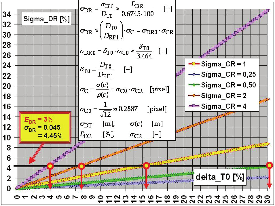
The last parameter that influences the size D RF1 is the length of the base b. Its size is selected
with respect to the demand for accomplishment of requisite size D T0 = D Tmax – the maximum
working range, in which the relative size of the probable error E DR of the range
measurement attains the given size, e.g. 3% – Fig. 11. The size of the base b depends
simultaneously on the size of the standard deviation σ( c) (resp. σC) of determination of the
disparity Δ c T corresponding to the range D Tmax.
Fig. 11. The main relations for estimate of POERF accuracy
As its basic (standardizing) value σC0 can be elected the standard deviation that originates
always in finding the integer value of the disparity Δ c T as an unrecoverable discretization
(quantizing) noise with the uniform distribution on the interval of the length just one pixel.
Then it is σC0 ≈ 0.2887 – Fig. 11. Instead of values σC, their relative values σCR can be used as
well. The value σC (resp. σCR) is the quality indicator for appropriate hardware and software
of the POERF, especially for algorithms for estimates of sizes of the disparity Δ c T under
given conditions (meteorological visibility, atmospheric turbulence, exposure time, aperture
ratio, motion blur, etc.). If the value of σCR increases twice, then it is necessary to elongate
the base b also twice with a view to preserve the requisite value D Tmax. Whence it follows
that the quality of hardware and software immediately influences the POERF sizes that are
directly proportional to the size of base b. The used base is 860 mm long.
The actual values of constants D RF1 and C 0RF are determined during manufacturing and
consecutively during operational adjustments. The adjustment is realized under utilization
Research and Development of the Passive Optoelectronic Rangefinder
337
of several targets whose coordinates are known for high accuracy. The appropriate
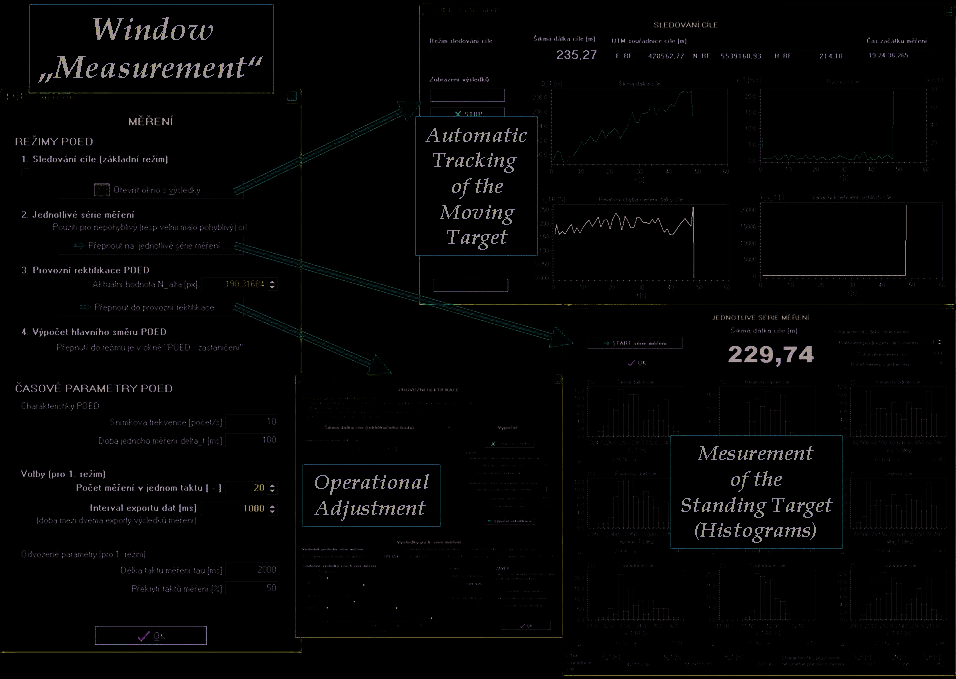
measurements are processed statistically with the use of the linear regress model (the
component part of POERF software – Fig. 14). For example, it was determined for targets 1
to 33 from the Catalogue of Targets (see the section 5, the Figures 16, 17) and for integer
estimates of the disparities that D RF1 = 9 215.5 m and C 0RF = 195.767 pixels (the correlation
coefficient r = − 0.999 725).
The starting situation in the process of a target searching and tracking can be characterized
as follows. The operator has only common information that a potentially interesting object
(the future target) could be in a given area. In the first period, the operator (sometimes with
the help of other persons) usually searches an odd object in the area under interest with his
eyes only or with the use of tools, e.g. field-glasses, and also with the help of POERF that
works in the regime “searching” in which the angles of view of the spotting camera are
sufficiently large (ideally c. 40° to 50°).
As soon as the target is identified and localized, the first period is closed and the second
period starts. The operator creates the first estimate of model of the target on the monitor
from the image provided by sighting camera (master) and passes on the computer. Sizes of
the first estimate of the target model must be sufficiently large – under aiming errors that
correspond to the actual situation and that are characterized by standard deviations in the
elevation σφ and in the traverse σψ – because the operator needs to place the real target into
the area of model of the target reliably – Fig. 12. Whenever he thinks that he attains it in the
process of sighting and tracking of the target, he pushes the appropriate button (Fig. 13) and
thus he passes the target model to the use in algorithms of automatic tracking of the target
and measuring of its range.
In the third period, the target position and its range are evaluated automatically. The
operator tries to reduce sizes of the target model (the POERF demonstration model 2009
does not enable it) and to place it again on the target. In the case of success, he pushes the
appropriate button and the system starts the exploitation of a new target model. The whole
process is supported by automatic stabilization of positions of optical axes of cameras and
eventually also by additional stabilization of the image on operator’s monitor (it is not
implemented in the demonstration model 2009). The operator can terminate this process as
soon as the target model includes pixels with only a part of image of the real target.
Complications are caused by objects which are situated in front of the target and are badly
visible, e.g. branches of bushes and trees, the grass, but also raised dust. The operator
consequently monitors automatically proceeding process. He enters into it in the case of
disappearance of the target behind a barrier for a longer time. In the case that information
about extrapolated future position of the target is exploited, a short disappearance of the
target can be compensated by the automatic system (not implemented in the demonstration
model 2009). The level of algorithm ability to learn will determine if the operator’s
intervention is needful in the case of the target turning to markedly other position towards
the POERF.
The program for automatic tracking of a target is based on the utilization of procedures
from the library Open CV, specifically on a modification of Lucas Kanade algorithm
(Bouguet, 1999). If the target disappears momentarily behind a barrier, then the algorithm
collapses. The operator must intervene as it is explained above.
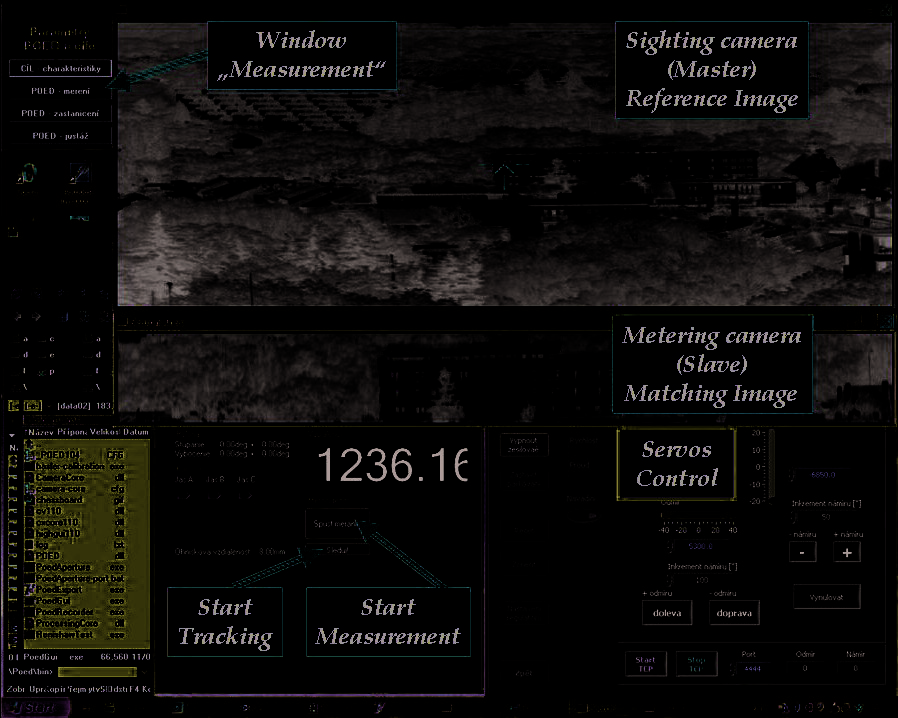
The program starts its functions as soon as the operator pushes the button “Start
Measurement” or “Start Tracking”. The algorithm then finds the nearest corner (of an object)
to the apex of the main aiming mark in the shot from the sighting camera. This point is
338
Optoelectronic Devices and Properties
considered the image T´1 of the target point T but only due to needs of the target tracking –
Fig. 9. Consequently, just two last consecutive shots from the sighting camera are processed.
With utilization of Lucas – Kanade Feature Tracker algorithm (Bouguet, 1999) for evaluation
of the optical flow, the position of the corner – the point T´1 – is always estimated in the
consequent shot with a subpixel accuracy. The algorithm is robust and that is why it can
cope with a gradual spatial slew of the target. The algorithm simultaneously highlights in
the image on the monitor the points, which have been identified as appurtenant to the
moving target, so that the operator has in his hands the screening control over the system
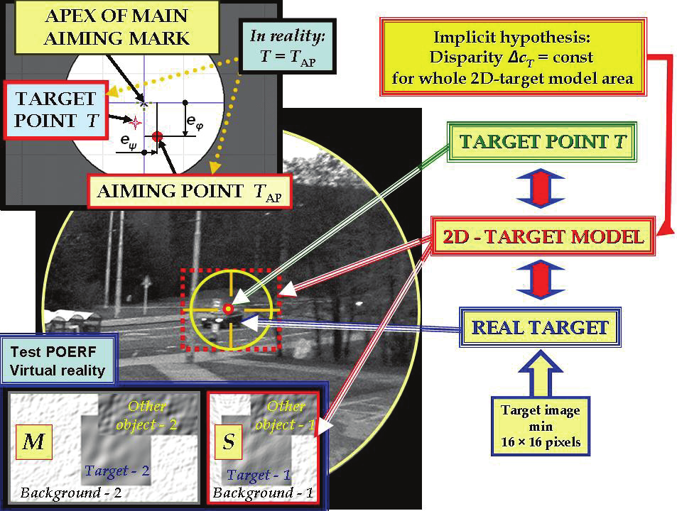
activity. In the case of problems, it is necessary to use 2D model of the target as mentioned
above. The point T´1 is at the same time considered the aiming point T AP – Fig. 12, and so the
control deviations ( eφ, eψ) are evaluated (as measured errors of angles) for the direction
channel control – Fig. 12.
Fig. 12. Relation among the image of the real target in the sighting camera, the target point T
and 2D model of the target
The maximum computing speed is required primarily, in order that about 30 range
measurements per second are necessary in our applications (POERF). Therefore, we prefer
simple (and hence very fast) algorithms. Random errors of measurements are compensated
during statistical treatment of measurement results (extrapolation process).
The matching cost function S( k) is used in the meantime (in general it is pixel-based
matching costs function) – the sum of squared intensity differences SSD (or mean-squared
error MSE) (Scharstein & Szelisky, 2002). The computation of matching cost function S( k)
proceeds in two steps.
Firstly, its global minimum with one-pixel accuracy is calculated (the tabulation over all
admissible horizontal shifts of the 2D target model on the matching image). Simultaneously,
Research and Development of the Passive Optoelectronic Rangefinder
339
the constriction for the choice of the global minimum – known as the Range Gate (Cech et
al., 2009) – is applied.
In the second step, the global minimum is searched with sub-pixel accuracy while using the
polynomial approximation (the interpolation and the least-squares method can be
alternatively used) in the neighbourhood of the integer point of the global minimum, which
has been found in the first step.
Fig. 13. Five basic windows for the operator during the target spotting, aiming and in the
beginning of the measurement or tracking
While using above-mentioned algorithms, it is always presumed that the same disparity
Δ c T = const is for all pixels of 2D target model – Fig. 12. This precondition is equivalent to
the hypothesis that these pixels depict immediate neighbourhood of the target point T
representing the target and this neighbourhood appertain to the target surface (more
accurately all that is concerned the image T’1 of this point and its neighbourhood). These
algorithms belong to the group referred to as local, fixed window based methods.
Adduced precondition can be frequently satisfied by a suitable choice of size and location of
the target model (i.e. by the aim of a convenient part of the target). The choice is performed
iteratively by the operator for the real POERF.
Usual shapes of a target surface (e.g. balconies on a building facade, etc.) have only a little
influence on the above-mentioned precondition violation, because the range difference
generated by them is usually less than 1 to 2 percent of the “average” target slant range D T
evaluated over the target surface represented by the 2D target model.
Operations over the set of pixels of the 2D target model that generate the matching cost
function S( k) and the procedure of its minimum searching can be counted as a definition of
special moving average, and – as a consequence – the whole process appears as a low-
frequency filtration.
340
Optoelectronic Devices and Properties
It holds generally that if respectively the meteorological visibility is low and the atmosphere
turbulence is strong, then it is necessary to choose a larger size of the 2D target model, i.e. to
filter out high spatial frequencies loaded by the largest errors and to work with lower spatial
frequencies.
Fig. 14. Auxiliary windows for monitoring of respectively the measurement and the
adjustment
In many cases it is inevitable that some pixels of the 2D target model record a rear object or a
front object instead of the target – Fig. 12. Simulation experiments with the program Test
POERF showed (Cech & Jevicky, 2007) that farther objects have minimal adverse impact on
the accuracy of the range measurement, contrary to nearer objects that induce considerably
large errors in the measurement of the target range. From the problem merits, these errors
are random blunders. Their greatness depends on the mutual position of the front object and
the target – Fig. 12. This finding has been also verified in computational experiments by the
help of the program RAWdis (Cech & Jevicky, 2010b). It is a specific particular case of more
common problem that is known as occluded areas; the specific case is the result of the depth
discontinuity (Zitnick & Kanade, 2000).
It is evident from the above that the choice of the position and the size of 2D target model is
not a trivial operation and it is convenient to entrust a man with this activity. The operator
introduces a priori and a posteriori information into the measurement process of
respectively the disparity and the range of a target and this information can be only hardly
(or not at all) obtained by the use of fully automatic algorithm.
Algorithms commonly published for the stereo correspondence problem solving are
altogether fully automatic – they use the information included in the given stereo pair
images, eventually in several consecutive pairs (optical flow estimation). Therefore, it is
possible to get inspired by these algorithms, but it is impossible to adopt them uncritically.
Research and Development of the Passive Optoelectronic Rangefinder
341
In conclusion it is necessary to state that these automatic algorithms are determined for
solving the dense or sparse stereo-problems, whereas the algorithms for POERF estimate the
disparity of the only point – the target point T, but under complicated and dynamically
varying conditions in the near-real-time.
4.2 Direction channel
The purpose of the direction channel is already mentioned above.
The core of the direction channel (Cech et al., 2009a) comprises two independent
servomechanisms for the elevation φ and the traverse ψ – Fig. 8. Identical servomotors and
servo-amplifiers by the firm TGdrives, s.r.o., Brno were used there. AC permanent magnet
synchronous motors (PMSM) TGH2-0050 (24 VDC) have a rated torque 0.49 Nm and a rated
speed 3000 rpm. The servo-amplifiers are of the type TGA-24-9/20. Furthermore, cycloidal
gearheads TWINSPIN TS – 60 from the firm Spinea, s.r.o., Presov with the reduction ratio
respectively 47 (elevation) and 73 (traverse) were used. Reduction ratio of the belt drive is
respectively 1.31 and 1.06.
The properties of the range channel and of the direction one are bound by the relation (Cech
et al., 2009)
c
δ
⋅ ρ( c)
θ = ω
Δ ⋅ t
max
Δ E_lag ≤θmax =
,
(3)
fa
where
θ max is the maximum permissible measurement error of the parallactic angle β – see the
Figure 9,
δc max is the same error expressed by pixels, e.g. δcmax = 0.1 (resp. 0.05) pixel,
Δ t E_lag is the absolute value of the time difference between starting the exposition in the
sighting camera and in the metering one,
Δ ω = | v Tp/ D T − ω S| is the absolute value of the error of the immediate angular velocity in the elevation/ traverse,
vTp is the appropriate vector component of the relative velocity of the target in the plane,
which is perpendicular to the radius vector of the target (i.e. perpendicular to the vector
determined by the points P RF and T),
ω S is the appropriate immediate angular velocity in the elevation/ traverse, which is
generated by the servo-drives.
It is evident from the relation (3) that the primary attention should be paid to the exact time
synchronization of expositions of the sighting camera and the metering one (resp. to the
synchronous sampling of the all relevant data), and that the increase of demands on the
precision of servo-drives is less important. It is interesting to retrace solutions of the
problem in former times (en.wikipedia/…/Base_end_station).
4.3 Target trajectory prediction
Algorithms used in the demonstration model POERF have been evolved by authors of this
chapter (Cech & Jevicky, 2009b). Consequently, they have created appropriate software.
Firstly, they developed a tuning and test simulation program and secondly, they have
programmed procedures for the library POED.DLL (these procedures are exploited by the
control program of POERF).
342
Optoelectronic Devices and Properties
Trigonometric calculations relate to points P RF (coordinates ( E, N, H)RF) and T (coordinates ( E, N, H)T), but rangefinder and target are spatial objects with nonzero sizes. It arises the fundamental problem, how and where to set unique contractual point on the rangefinder,
and analogously, how and where to set (preferably uniquely) contractual point on the area
of target image in the sight.
Chosen position of the point T in the target image determines simultaneously its position in
the space. This point T is conventionally described as the “target point”, i.e. reference point
that represents the target at given moment due to needs of measurement of the target
position.
Rangefinder construction can require aiming by the sight not into the target point T, but into
so-called “aiming point” T AP. Its position must be chosen in accordance with instructions for
the work with rangefinder. In our case, the aiming point T AP is identical with the target
point T – Fig. 12.
As a result of aiming errors (Fig. 12), the position of the apex of the main aiming mark in the
rangefinder sight (that represents the position of sensitive axis of the rangefinder in the
space) does not coincide with the position of the aiming point T AP image in the sight at the
moment of range measurement. It is usually the source of additional errors in measurement
of the target position in the space because the range to the point Tís measured (and it is
possible that this point lies off the target), but the range is interpreted as range to the target
point T. In this case, a gross error appears in the target range measurement.
By reason of simple derivation of seeking dependencies, it is necessary to introduce several
coordinate systems. Detailed analysis of this problem was already presented in (Cech et al.,
2009a).
The measurement point ( j-th point of measurement Tj = T(tj) denotes position of the target
point T at the moment tj that characterizes contractually the moment of taking the stereo-
pair images, from which the target slant range D Tj is evaluated.
Data record ( j-th record) – means a process beginning by preparation for taking the stereo-
pair images (time t START j = t S j) and ending (time t STOP j = t K j) by completion of export of evaluated estimate of the target coordinates (generally ( E, N, H)T j), that are contractually related to the “measurement moment”, i.e. in the time t STOP j, the target coordinates are given
to the next use for all system. The length of record continuance is T Z j = t STOP j – t START j.
Observing period is the time interval between two consecutive records (exports of data – the
target coordinates) t OP j = t K j – t K j–1. This period is usually constant, t OP j = t OP = const.
On the basis of information from publications and supposed accuracy of the test device
POERF, the linear hypothesis about target motion was selected (presumption of uniform
straight-line motion of the target with constant speed) as the most robust hypothesis from
applicable ones. This hypothesis, in the case of immovable target, degenerates automatically
into hypothesis of stationary target. Measured data are smoothed by linear regress model.
Application of Kalman filter is problematic enough, especially due to low frequency of the
target slant range measurement. This frequency is c. 10 to 100 times lower than it is usual in
radiolocation. Needful organization of all processes follows from adduced preconditions –
Fig. 15.
Total Nk data records – measurements ( j = j min k, … , j max k) are evaluated together in the k-th cycle. In our model there is Nk = const for k = 2, 3, … and N 1 = N 2·P1,0. Linear regress model is applied on data from these records.
One measurement period Δ t MES1, as the interval between two successive measurement
points, is estimated from the rate frame [fps]. Measurement cycles overlap Pk, k-1 = 1 –
Research and Development of the Passive Optoelectronic Rangefinder
343
( N SH k/ Nk) is in functional relation with the interval of data export T SH k. The overlap of measurement cycles denotes what relative number of records (measurements) is shared by
two successive cycles.
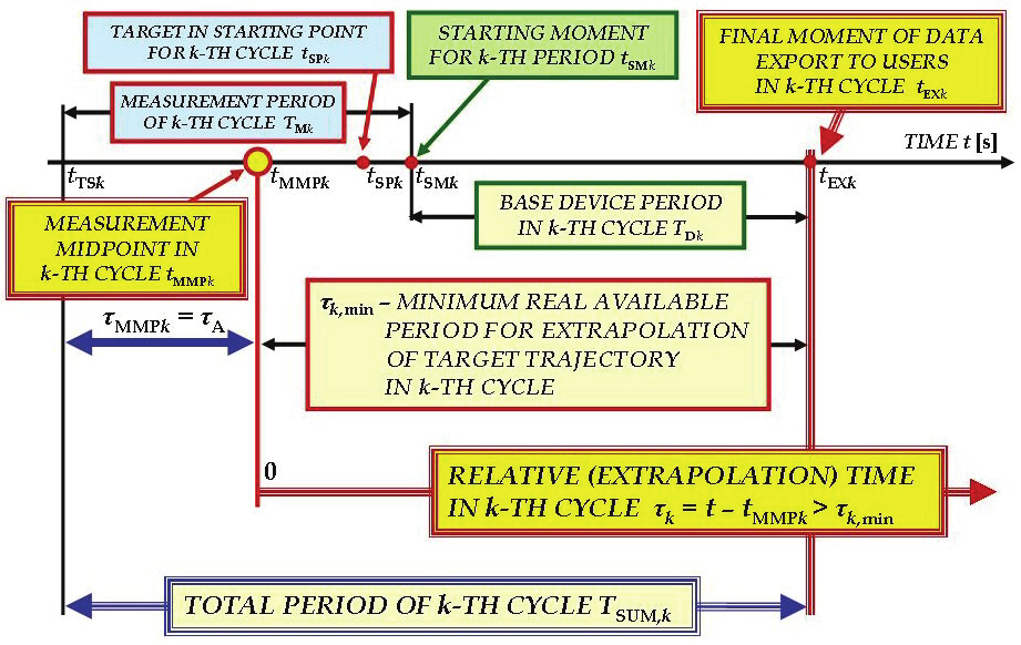
Fig. 15. Fundamental relations among time data needful for the target trajectory
extrapolation
Two terms refer to the last record used in the k-th cycle. At the moment of taking the la