50
100
150
200
Autocorrelation of the signal O -5 Point3 INOE
3
2000
Power=1877.9064
1500
2
1000
ppb
500
0
-200
-150
-100
-50
0
50
100
150
200
Delay
Fig. 16. Typical autocorrelation functions
Statistical Tools and Optoelectronic Measuring Instruments
427
The sample auto covariance, C [ l] , is the sample autocorrelation of the centred sequence
xx
[ x ] (the sequence after removing the mean) while the sample cross covariance, C [ l] , is the i
xy
cross correlation of the centred sequences [ x ] and [ y ] . Thus, Fig. 17 presents the auto
i
i
covariance functions for the same signals, namely Point1UPT and Point3INOE pollutant
concentrations. The auto covariance at zero lag, gives the power of the variable part of the
analysed signal: approximately 74 ppb 2 for Point1UPT and 131 ppb 2 for Point3INOE signals.
The shapes of the auto covariance functions show that Point1UPT signal has a highly
random character while in the Point3INOE signal the spectral components are concentrated
in a small range near 0.016 mHz.
Autocovariance of the signal O -5 Point1 UPT
3
80
Power=73.9371
60
40
2
ppb
20
0
-20
-200
-150
-100
-50
0
50
100
150
200
Autocovariance of the signal O -5 Point3 INOE
3
150
Power=130.5687
100
2
50
ppb
0
-50
-200
-150
-100
-50
0
50
100
150
200
Delay
Fig. 17. Typical auto covariance functions
The cross-covariance functions offer an interesting possibility to determine delays between
pollutant concentrations measured simultaneously. The position of the peak in the
covariance function around zero gives the temporal delay between two signals. Depending
on the wind direction and intensity the pollutants can be transported from one place to the
other in the experimental area. However such temporal relations can be put into evidence
only if the resolution on the time axis is sharp enough to allow the proper localization of the
crosscovariance peak. This condition was not fulfilled during the related measuring
campaign: the sampling period should be in the range of seconds while the signals were
achieved with sampling periods of 5 to 30 minutes. The consequence is that the peak of the
autocorrelation function appears in the origin (zero lag) or they have a flat maximum
around zero, as shown in Fig.18.
Summarizing, the autocorrelation and auto-covariance functions are useful tools in
establishing power relations between pollutant concentration signals measured with
428
Optoelectronic Devices and Properties
optoelectronic instruments. For reliable results, a sufficient temporal length of measured
data sets must be assured, so that the signals can manifest there features. Temporal relations
i.e. delays between certain signals measured simultaneously can be revealed using the
crosscovariance function. But, for this purpose a supplementary condition must be fulfilled:
a small sampling period must assure a good resolution on the time axis.
Crosscovariance of the signals O -5 Point1 UPT and Point3 INOE
3
80
60
40
2
20
ppb
0
-20
Value at Zero Delay=67.7611
-40
-200
-150
-100
-50
0
50
100
150
200
Cosscovariance of the signals O -5 Point1 UPT and DOAS1 INOE
3
60
40
20
2
ppb
0
-20
Value at Zero Delay=54.254
-40
-200
-150
-100
-50
0
50
100
150
200
Delay
Fig. 18. Experimental cross covariance functions
The MATLAB xcorr function produces estimates of the cross-correlation function. For
example, the command C=xcorr(A,B), where A and B are length M vectors, returns the length 2* M- 1 crosscorrelation sequence C. Particularly, C=xcorr(A), where A is a vector, returns the autocorrelation sequence. One can limit the range of lags in the (auto/cross)
correlation function to (- Maxlag, Maxlag), using the command form xcorr(...,Maxlag).
Similarly, the MATLAB function xcov produces estimates of the (auto/cross) covariance
function (actually, correlation functions of sequences with their means removed).
6. Conclusion
Due to the random character of the pollutant concentrations measured with optoelectronic
instruments, statistical signal processing methods are recommended. Histograms,
correlation coefficients, (auto/cross) correlation, (auto/cross) covariance functions or
statistical parameters like mean, standard deviation, skewness and kurtosis can be useful
tools in analyzing such signals. However, according to the purpose of the measuring
campaign, the experiment must be carefully designed in order to obtain reliable results.
This chapter reveals some practical rules for setting acquisition parameters like data
Statistical Tools and Optoelectronic Measuring Instruments
429
(segment) size and sampling frequency. As a first rule, for reliable correlation coefficient
determination one must assure a sufficient temporal length of the concentration signals,
i.e. the product between segment size and sampling period must be large enough in order
to obtain stable values of the correlation coefficients. This rule is also valid for the
calculation of autocorrelation or auto covariance functions. However, if we are interested
to use cross correlation or cross covariance function to reveal delays between pollutant
concentration and/or meteorological signals, another rule must also be taken into
account: assure the necessary resolution on the time axis i.e. the sampling period must be
small enough in comparison with expected delays. In any case, interactive verification
and setting of the acquisition parameters during the measuring campaign, according to
the purpose of every particular experimental research, are recommended.
Signal conditioning procedures must be implemented before determining the statistical
functions and parameters. Thus, ideal filtering based on fast Fourier transform is an
useful pre-processing step allowing a simple rejection of measurement noise and possible
artefacts of the pollution level signals. Interpolation can be used to increase the number of
samples of the slowly varying meteorological parameters, avoiding redundant
measurements.
The purpose of one measuring campaign was the correlative comparison of two CO-
concentration optoelectronic measuring instruments, working on different principles.
Within this research the correlation coefficient proved to be the most useful tool in
analyzing dependencies between pollution levels and the meteorological factors. The
open path remote sensing instrument measures spatial averaged values which show
better correlation to the meteorological parameters. Thus, the open path instrument is
better suited for monitoring the pollution level in a large area than the classical NDIR
device.
7. References
Hoffmann, J. & Quint, F. (2007). Signalverarbeitung mit MATLAB® und SIMULINK®.
Anwendungsorientierte Simulationen, Oldenbourg Verlag, ISBN 978-3-486-58427-1,
München
Ionel, I.; Ionel, S. & Nicolae, D. (2007). Correlative comparison of two optoelectronic carbon
monoxide measuring instruments. Journal for Optoelectronics and Advanced Materials,
Vol. 9, No. 11, pp. 3541-3545 ISSN
Ionel, I.; Ionel, S. & Lie, I. (2009). Statistical Tools in the Analysis of Pollutant Concentrations
Measured with Optoelectronic Instruments, Proceedings of the 11th WSEAS
International Conference on Sustainability in Science and Engineering (SSE ’09), Vol. II,
pp.293-298, Timişoara, Romania, May, 2009, Published by WSEAS Press
Martinez, L. W. & Martinez, R. A. (2002). Computational Statistics Handbook with MATLAB®,
Chapman & Hall/CRC, ISBN 1-58488-229-8, Boca Raton
Montgomery, C. D. & Runger, C. G. (2006). Applied Statistics and Probability for Engineers, 4th
Edition, John Wiley & Sons, Inc., ISBN 0-471-74589-8, New York
Navidi, W. (2010). Statistics for Engineers and Scientists, McGraw-Hill, Inc., 3rd Edition, ISBN-
13: 978-0071222051, New York
Papoulis, A. (1991). Probability, Random Variables, and Stochastic Processes, McGraw-Hill, Inc.,
3rd Edition, ISBN 0-07-100870-5, New York
430
Optoelectronic Devices and Properties
Peck, R.; Olsen, C. & Devore, J. (2008). Introduction to Statistics and Data Analysis, Duxbury
Press, 3rd Edition, ISBN-13: 978-0-495-11873-2, Pacific Grove, CA
Shen, D.; Lu, Z. (2006). Computation of Correlation Coefficient and Its Confidence Interval
in SAS, www2.sas.com/proceedings/sugi31/170-31.pdf
Therrien, C. W. (1992). Discrete Random Signals and Statistical Signal Processing, Prentice-Hall
International, Inc., ISBN 0-13-217985-7, Englewood Cliffs
Zuur, A. F.; Ieno, E. N. & Smith, G. M. (2007). Analyzing Ecological Data, Springer Science +
Business Media, ISBN-13: 978-0-387-45967-7, New York
Part 5
Physical Modeling and Simulations
of Optoelectronic Devices
21
Advanced Numerical Simulation
of Organic Light-emitting Devices
Beat Ruhstaller1, Evelyne Knapp2, Benjamin Perucco3, Nils Reinke4,
Daniele Rezzonico5 and Felix Müller6
1,2,3,4 Zurich University of Applied Sciences, Institute of Computational
Physics, 8401 Winterthur
5,6 Fluxim AG, 8835 Feusisberg
Switzerland
1. Introduction
Organic light-emitting devices (OLEDs) are novel and efficient light sources that consist of a
sequence of layers that fulfill distinct electronic and optical tasks. Given the variety of organic
semiconductor materials available, the improvement of the device performance is a tedious
and demanding task that often involves numerous experimental optimizations of layer
materials, thicknesses and sequence. Comprehensive numerical device models have recently
been developed that master both the physical complexity of the underlying optoelectronic
processes as well as the numerically challenging system of equations. In this chapter we
introduce such a comprehensive optical and electronic device model that is able to describe the
device performance of OLEDs. We first introduce the key device model equations for charge
and exciton transport as well as the dipole emission model for describing the out-coupling
of light. Then we present a series of simulation results that are of practical interest when
studying and optimizing OLEDs. These include the calculation of current-voltage curves,
current transients signals, time-of-flight current transients and impedance spectroscopy data.
We show that the physical model can be combined with a nonlinear least-square fitting
algorithm for extracting transport parameters from measurements. In terms of optical device
characteristics, quantitative outcoupling mode contributions and angular characteristics are
presented as well as results of an emission zone extraction method.
Electrical characterization of devices and materials is essential and helps to elucidate
the underlying, physical models of charge carrier transport in disordered, organic
semiconductors.
Besides the commonly used current-voltage curves, dark-injection,
electroluminescence and time-of-flight transient measurements as well as impedance
spectroscopy offer other ways to validate models for organic LEDs and extract model
parameters. By means of a one-dimensional numerical OLED model we are able to simulate
these different measurement techniques. Here, we present numerical methods in the physical
and numerical framework of reference (Knapp et al, 2010) and solve directly for the steady-
and transient state. Further, we conduct a numerical small signal-analysis for OLEDs. The
underlying model solves the drift-diffusion equations in a coupled manner for disordered,
434
Optoelectronic Devices and Properties
organic semiconductors. The disordered nature of organic semiconductors affects the density
of state, the mobility model, the Einstein diffusion relation as well as charge injection.
These novel physical model ingredients constitute a second generation OLED model and are
implemented in the simulator SETFOS (Fluxim AG, 2010). It is expected that the second
generation OLED model will impact the way OLED characteristics and performance are
quantitatively described.
2. Description of the device model
2.1 Charge drift-diffusion model
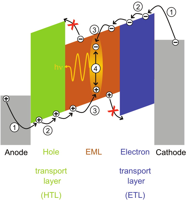
To describe the main features of charge transport in organic LEDs four processes have to be
considered as illustrated in the schematic energy level diagram in Fig. 1. In a first step, charge
carriers have to be injected into the organic material (1), secondly they will be transported (2)
until they recombine to an exciton (3). Then the excitons decay radiatively or non-radiatively
(4). In the following we will first look at the transport process (2). For the description of
Fig. 1. Main processes in OLED operation: 1) Injection, 2) Transport, 3) Formation of exctions,
4) Radiative decay
charge transport in OLEDs the general semiconductor drift-diffusion equations for electrons
and holes are valid. In Poisson’s equation
∇ · ( ∇ψ) = e( n + nt − p − pt),
(1)
the electrical potential ψ is related to the mobile electron and hole densities n and p and the trapped electron and hole densities nt and pt where e is the elementary charge and
the
product of the vacuum permittivity 0 and the relative permittivity r of the organic material.
The current equations for electrons and holes read
Jn = −enμn∇ψ + eDn∇n,
(2)
Jp = −epμp∇ψ − eDp∇p
Advanced Numerical Simulation of Organic Light-emitting Devices
435
where μn, p denotes the mobility and Dn, p the diffusion coefficient for electrons and holes. Only mobile charges contribute to the current. The conservation of charges leads to the continuity
equations for electrons and holes
∂n
∂ = 1 ∇J
,
t
e
n − R( n, p) − ∂nt
∂t
∂p
(3)
∂ = − 1 ∇J
t
e
p − R( n, p) − ∂pt
∂t
where R denotes the bimolecular recombination rate given by Langevin and t the time
(Langevin, 1903). These equations take charge migration and recombination into account. The
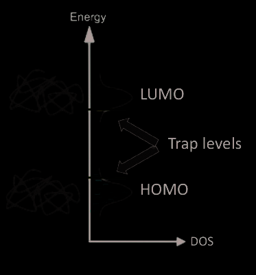
trapped electron ( nt) and hole ( pt) charge carriers obey the rate equations for an energetically
sharp trap levels as shown in Fig. 2
∂nt
∂ = r
t
cn( Nt − nt) − rent,
∂p
(4)
t
∂ = r
t
c p( Nt − pt) − re pt.
where re denotes the escape rate, rc the capture rate and Nt the trap density. Note, that more general trap distributions can be introduced that are described by an exponential or Gaussian
density of trap states (Fluxim AG, 2010; Knapp et al, 2010).
Fig. 2. Gaussian distributions of density of states and trap levels for trapped charges.
As opposed to inorganic semiconductors the density of states for organic semiconductors is
described by a Gaussian shape since transport is assumed to occur via a hopping process
between uncorrelated sites. Thus, polymers and small molecules have broadened energy
levels of their highest occupied molecular orbital (HOMO) and lowest unoccupied molecular
orbital (LUMO) as shown in Fig. 2 and are described in the following way
2
NGauss( E) =
N 0
√
exp −
E − E 0
√
(5)
2 πσ 2
2 σ
where N 0 denotes the site density, σ the width of Gaussian and E 0 the reference energy
level. In the extended Gaussian disorder model the Gaussian density of states affects charge
diffusion. Tessler pointed out that the use of the generalized instead of the classical Einstein
436
Optoelectronic Devices and Properties
relation is appropriate (Tessler et al., 2002). The generalized Einstein diffusion coefficient is
now determined by
D = kT μ( T, p, F) g
q
3( p, T),
(6)
where the enhancement function g 3 reads
p
g 3( p, T) = 1
.
(7)
kT ∂p
∂Ef
Using the expression
∞
p( Ef ) =
DOS( E) f ( E, E
−∞
f ) dE
(8)
for the density and inserting the Fermi-Dirac distribution and the Gaussian DOS we obtain
∞
NGauss( E)
1
dE
E−E f
D
−∞
1+exp
= kT
kT
μ
.
(9)
q
E−E f
∞ NGauss( E) exp
kT
−∞
dE
[
E−E
1+exp
f
]2
kT
We will now turn to the charge mobility model. A mobility model that has been applied for
quite some time now is the Poole-Frenkel mobility which is field-dependent and reads
√
μ = μ 0 exp γ E ,
(10)
where μ 0 is the zero-field mobility and γ is the field-dependence parameter. However, it has
been shown by Bässler with the aid of Monte Carlo simulations that the energetic disorder in
organic semiconductors influences the charge mobility (Pautmeier et al., 1990). Experiments
have shown that the mobility in hole-only devices can differ up to three orders of magnitude
between OLED and OFET device configurations with the same organic semiconductor. An
explanation for this difference is a strong dependence of the mobility on the charge density
(Tanase et al., 2003). Vissenberg and Matters developed a mobility model that considers
such a density-dependent effect (Vissenberg & Matters, 1998). Using a 3D master equation
approach to simulate the hopping transport in disordered semiconductors a dependence on
the temperature, field and density was determined. Pasveer’s model is therefore dependent
on the temperature, field as well as the density and accounts for the disorder in the material
(Pasveer et al, 2005). The extended Gaussian disorder model (EGDM) is an extension of the
Pasveer model by additionally considering diffusion effects. In the EGDM the mobility may
be expressed as a product of a density-dependent and field-dependent factor according to van
Mensfoort as (Mensfoort et al., 2008a)
μ( T, p, F) = μ 0( T) g 1( p, T) g 2( F, T), (11)
with the enhancement functions g 1( p, T) and