parts can be measured because the gripper covers half of the guide and the stator (see Fig. 12
Size-adapted Parallel and Hybrid Parallel Robots for Sensor Guided Micro Assembly
241
right). Therefore, the 3D vision sensor observes only the visible sides of the assembled parts.
This means that the measured positioning error and the resulting positioning uncertainty
are only determined by the visible part side. After the process, both ends of the assembly
group can be inspected and the overall assembly deviation can be measured. The assembly
uncertainty is calculated from the deviations. This value is comprised of the overall errors
during the assembly of the micro system.
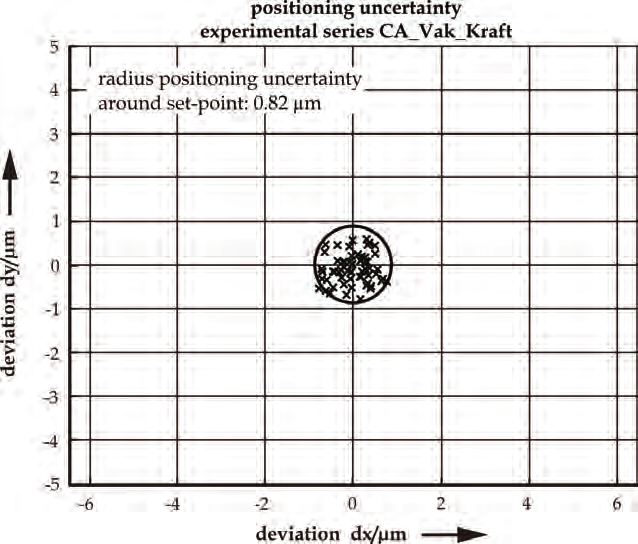
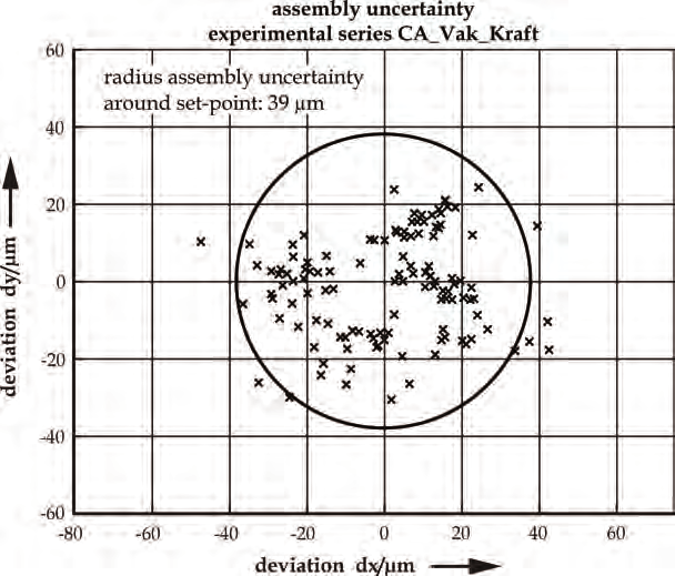
An assembly uncertainty of 38 µm and a positioning uncertainty of 0.82 µm are reached for
the assembly process. The difference between assembly uncertainty and positioning
uncertainty is a result of the relatively long part length of 10.66 mm. A small angular
deviation causes a positioning error (in xy-direction). This error is larger at the side of the
part which is invisible during the positioning process than the error on the visible side. With
a greater part length, this positioning error will be higher than with smaller parts.
Furthermore, deviations occurring during the bonding process cause an increased assembly
error. Figure 14 shows the positioning uncertainty and figure 15 the assembly uncertainty of
the assembled groups. The circles in the diagrams show the radius of the uncertainties.
Fig. 14. Reached positioning uncertainty
In another assembly task, assembly uncertainties of 25 µm were reached with another
design of the assembly group. Therefore, the distance between the positioning marks has
been enlarged. A positioning uncertainty and a limit value of 0.5 µm was reached with this
arrangement of the positioning marks. This demonstrates the potential for further
improvement of the assembly uncertainty.
242
Parallel Manipulators, Towards New Applications
Fig. 15. Reached assembly uncertainty
4. Conclusion
Micro assembly tasks demand low assembly uncertainties in the range of a few
micrometers. This request results from the small part sizes in the production of MST
components and the resulting small valid tolerances. Since precision robots represent the
central component of an assembly system, an appropriate kinematic structure is crucial.
These kinematic structures can be serial, parallel or hybrid (serial/parallel). Although serial
structures can be used for micro assembly, they have large moved masses and need a
massive construction of the frame and robot links to obtain an appropriate repeatability.
Therefore, some size-adapted parallel and hybrid parallel robot structures were presented in
the previous sections. Very good repeatabilities were reached with the presented robots due
to the chosen structures, the miniaturized design and the use of flexure hinges as ultra-
precision machine components.
Besides the precision robot, most assembly tasks require the use of additional sensors with
high resolutions and measurement accuracies to reach a low assembly uncertainty.
Therefore, optical and/or force sensors are used for sensor guided micro assembly
processes.
The terms “absolute sensor guidance” and “relative sensor guidance” were introduced. Both
methods offer an enhancement of the accuracy within micro assembly processes. The
“relative sensor guidance” promises a lower positioning and assembly uncertainty because
of the user defined number of position correction loops. Therefore, relative sensor guidance
was used in the presented example for micro assembly.
Size-adapted Parallel and Hybrid Parallel Robots for Sensor Guided Micro Assembly
243
With the use of relative sensor guidance, positioning uncertainties below 0.5 µm can be
reached. The assembly uncertainty has to be further improved to fulfil the demand for
assembly uncertainties in the range of a few micrometers. Therefore, the design of the
product and positioning marks as well as the gripping and joining technology has to be
examined in future developments.
5. References
Berndt, M. (2007). Photogrammetrischer 3D-Bildsensor für die automatisierte Mikromontage,
Schriftenreihe des Institutes für Produktionsmesstechnik, No. 3, Shaker Verlag,
ISBN 978-3-8322-6768-1, Aachen
van Brussel, H. ; Peirs, J. ; Delchambre, A. ; Reinhart, G. ; Roth, N. ; Weck, M. & Zussman, E.
(2000). Assembly of Microsystems, Annals of CIRP, Vol. 49, No. 2, pp. 451-472
Clavel, R.; Helmer, P.; Niaritsiry, T.; Rossopoulos, S.; Verettas, I. (2005). High Precision
Parallel Robots for Micro-Factory Applications, Robotic Systems for Handling and
Assembly - Proc. of 2nd International Colloquium of the Collaborative Research Center 562,
Fortschritte in der Robotik Band 9, Shaker Verlag, ISBN 3-832-3866-2, Aachen,
pp. 285-296
Coudourey, A.; Perroud, S.; Mussard, Y. (2006). Miniature Reconfigurable Assembly Line
for Small Products, Proc. Third International Precision Assembly Seminar (IPAS'2006),
Springer Verlag, ISBN 0-387-31276-5, Berlin, pp. 193-200
DIN ISO 230-2 (2000). Prüfregeln für Werkzeugmaschinen, Teil 2: Bestimmung der
Positionierunsicherheit und der Wiederholpräzision der Positionierung von
numerisch gesteuerten Achsen, Beuth Verlag, Berlin
EN ISO 9283 (1999). Industrieroboter: Leistungskenngrößen und zugehörige Prüfmethoden.
Beuth Verlag, Berlin
Fatikow, S. (2000). Miniman. In: Mikroroboter und Mikromontage, p. 277, Teubner Verlag,
ISBN 3-519-06264-X, Stuttgart – Leipzig
Hesselbach, J.; Plitea, N. ; Thoben, R. (1997). Advanced technologies for micro assembly,
Proc. of SPIE, Vol. 3202, pp. 178-190
Hesselbach, J. ; Raatz, A. (2000). Pseudo-Elastic Flexure-Hinges in Robots for Micro
Assembly, Proc. of SPIE, Vol. 4194, pp. 157-167
Hesselbach, J. ; Raatz, A. & Kunzmann, H. (2004a). Performance of Pseudo-Elastic Flexure
Hinges in Parallel Robots for Micro-Assembly Tasks, Annals of CIRP, Vol. 53, No. 1,
pp. 329-332
Hesselbach, J.; Wrege, J.; Raatz, A.; Becker, O. (2004b) Aspects on Design of High Precision
Parallel Robots, Journal of Assembly Automation, Vol. 24, No. 1, pp. 49-57
Hesselbach, J. ; Wrege, J. ; Raatz, A. ; Heuer, K. & Soetebier, S. (2005). Microassembly -
Approaches to Meet the Requirements of Accuracy, In : Advanced Micro &
Nanosystems Volume 4 - Micro-Engineering in Metals and Ceramics Part II, Löhe, D.
(Ed.) & Haußelt, J. (Ed.), pp. 475-498, Wiley-VCH Verlag, ISBN 3-527-31493-8,
Weinheim
Höhn, M. (2001). Sensorgeführte Montage hybrider Mikrosysteme, Forschungsberichte iwb,
Herbert Utz Verlag, ISBN 3-8316-0012-0, München
Howell, L.L. ; Midha, A. (1995). Parametric Deflection Approximations for End-Loaded,
Large-Deflection Beams in Compliant Mechanisms, Journal of Mechanical Design,
Vol. 117, No. 3, pp. 156-165
244
Parallel Manipulators, Towards New Applications
Paros, J.M. ; Weisbord, L. (1965). How to Design Flexure Hinges, Machine Design, Vol. 25,
pp. 151-156
Raatz, A. (2006). Stoffschlüssige Gelenke aus pseudo-elastischen Formgedächtnislegierungen in
Parallelrobotern, Vulkan Verlag, ISBN 3-8027-8691-2, Essen
Raatz, A. & Hesselbach, J. (2007). High-Precision Robots and Micro Assembly, Proceedings of
COMA ’07 International Conference on Competitive Manufacturing, pp. 321-326,
Stellenbosch, South Africa, 2007
Simnofske, M. ; Schöttler, K. ; Hesselbach, J. (2005). Micabof2 – robot for micro assembly,
Production Engineering, Vol. 12, No. 2, pp. 215-218
Smith, S.T. (2000). Flexures - Elements of Elastic Mechanisms. Gordon & Breach Science
Publishers, ISBN 90-5699-261-9, Amsterdam
Tutsch, R.; Berndt, M. (2003). Optischer 3D-Sensor zur räumlichen Positionsbestimmung bei
der Mikromontage, Applied Machine Vision, VDI-Report No. 1800, Stuttgart, pp. 111-
118
Wicht, H. & Bouchaud, J. (2005). NEXUS Market Analysis for MEMS and Microsystems III
2005-2009, mst news, Vol. 5, 2005, pp. 33-34
12
Dynamics of Hexapods with Fixed-Length Legs
Rosario Sinatraa and Fengfeng Xib
aUniversità di Catania, 95125, Catania,
bRyerson University Toronto, Ontario,
aItaly
bCanada
1. Introduction
Hexapod is a new type of machine tool based on the parallel closed-chain kinematic
structure. Compared to the conventional machine tool, parallel mechanism structure offers
superior stiffness, lower mass and higher acceleration, resulting from the parallel structural
arrangement of the motion systems. Moreover, hexapod has the potential to be highly
modular and re-configurable, with other advantages including higher dexterity, simpler and
fewer fixtures, and multi-mode manufacturing capabilities.
Initially, hexapod was developed based on the Stewart platform, i.e. the prismatic type of
parallel mechanism with the variable leg length. Commercial hexapods, such as VARIAX
from Giddings & Lewis, Tornado from Hexel Corp., and Geodetic from Geodetic
Technology Ltd., are all based on this structure. One of the disadvantages for the variable
leg length structure is that the leg stiffness varies as the leg moves in and out. To overcome
this problem, recently the constant leg length hexapod has been envisioned, for instance,
HexaM from Toyada (Susuki et al., 1997). Hexaglibe form the Swiss Federal Institute of
Techonology (Honegger et al., 1997), and Linapod form University of Stuttgart (Pritschow &
Wurst, 1997). Between these two types, the fixed-length leg is stiffer (Tlusty et al., 1999) and,
here, becoming popular.
Dynamic modeling and analysis of the parallel mechanisms is an important part of hexapod
design and control. Much work has been done in this area, resulting in a very rich literature
(Fichter, 1986; Sugimoto, 1987; Do & Yang, 1988; Geng et al., 1992; Tsai, 2000; Hashimoto &
Kimura, 1989; Fijany & Bejezy, 1991). However, the research work conducted so far on the
inverse dynamics has been focused on the parallel mechanisms with extensible legs.
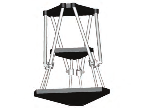
In this chapter, first, in the inverse dynamics of the new type six d.o.f. hexapods with fixed-
length legs, shown in Fig. 1, is developed with consideration of the masses of the moving
platform and the legs. (Xi & Sinatra, 2002) This system consists of a moving platform MP
and six legs sliding along the guideways that are mounted on the support structure. Each
leg is connected at one end to the guideway by a universal joint and at another end to the
moving platform by a spherical joint. The natural orthogonal complement method (Angeles
& Lee, 1988; Angeles & Lee, 1989) is applied, which provides an effective way of solving
multi-body dynamics systems. This method has been applied to studying serial and parallel
manipulators (Angeles & Ma, 1988; Zanganesh et al., 1997) automated vehicles (Saha &
Angeles, 1991) and flexible mechanisms (Xi & Sinatra, 1997). In this development, the
246
Parallel Manipulators, Towards New Applications
Newton-Euler formulation is used to model the dynamics of each individual body,
including the moving platform and the legs. All individual dynamics equations are then
assembled to form the global dynamics equations. Based on the complete kinematics model
developed, an explicit expression is derived for the natural orthogonal complement which
effectively eliminates the constraint forces in the global dynamics equations. This leads to
the inverse dynamics equations of hexapods that can be used to compute required actuator
forces for given motions.
Fig. 1. New hexapod design
Finally, for completeness of the dynamic study of the parallel manipulator with the fixed-
length legs, the static balancing is studied (Xi et al., 2005).
A great deal of work has been carried out and reported in the literature for the static
balancing problem. For example, in the case of serial manipulator, Nathan (Nathan, 1985)
and Hervé (Hervé, 1986) applied the counterweight for gravity compensations. Streit et al.
(Streit & Gilmore, 1991), (Walsh et al., 19) proposed an approach to static balanced rotary
bodies and two degrees of freedom of the revolute links using springs. Streit and Shin
presented a general approach for the static balancing of planar linkages using springs(Streit
& Shin, 1980). Ulrich and Kumar presented a method of passive mechanical gravity
compensation using appropriate pulley profiles (Ulrich & Kumar, 1991). Kazerooni and Kim
presented a method for statically-balanced direct drive arm (Kazerooni & Kim, 1990).
For the parallel manipulator much work was done by Gosselin et al. Research reported in
(Gosselin & Wang, 1998) was focused on the design of gravity-compensated of a six–degree-
of-freedom parallel manipulator with revolute joints. Each leg with two links is connected
by an actuated revolute joint to the base platform and by a spherical joints the moving
platform. Two methods are used, one approach using the counterweight and the other using
springs. In the former method, if the centre of mass of a mechanism can be made stationary,
the static balancing is obtained in any direction of the Cartesian space. In the second
approach, if the total energy is kept constant, the mechanism is statically balanced only in
the direction of gravity vector. The static balancing conditions are derived for the three-
degree-of-freedom spatial parallel manipulator (Wang & Gosselin, 1998) and in similar
Dynamics of Hexapods with Fixed-Length Legs
247
conditions are obtained for spatial four-degree-of-freedom parallel manipulator using two
common methods, namely, counterweights and springs (Wang & Gosselin, 2000).
In this chapter, following the same approach presented by Gosselin, the static balancing of
the six d.o.f. platform type parallel manipulator with the fixed-length legs shown is studied.
The mechanism can be balanced using the counterweight with a smart design of
pantograph. The mechanism can be balanced using the method, i.e., the counterweight with
a smart design of pantograph. By this design a constant global center of mass for any
configurations of the manipulator is obtained.
Finally, the leg masses become important for hexapods operating at high speeds, such as
high-speed machining; then in the future research and development the effect of leg inertia
on hexapod dynamics considering high-speed applications will be investigated.
2. Kinematic modeling
2.1 Notation
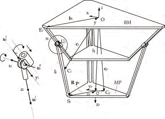
As shown in Figure 2, this hexapod system consists of a moving platform MP to which a
tool is attached, and six legs sliding along the guideways that are mounted on the support
structure including the base platform BP. Each leg is connected at one end to the guideway
by a universal joint and at another end to the moving platform by a spherical joint.
Fig. 2. Kinematic notation of the i th leg
The coordinate systems used are a fixed coordinate system O-xyz is attached to the base and
a local coordinate system O t- xtytzt attached to the moving platform. Vector b i, s i, and l i are directed from O to B i, from B i to U i, and from U i to S i respectively. B i indicates the position of one end of the i th guideway attached to the base, U i indicates the position of the i th
248
Parallel Manipulators, Towards New Applications
universal joint, and Si indicates the position of the i th spherical joint. Six legs are numbered
from 1 to 6.
Furthermore, a local coordinate frame O i-x i y i z i is defined for each leg, with its origin located
at the center of the i th universal joint. Two unit vectors are used. Unit vector l
u i is along the
leg length representing the direction of the i th leg, and unit vector s
u i is along the guideway
representing the direction of the i th guideway. The orientation of the i th coordinate frame
with respect to the base can therefore be defined by a 3 × 3 rotation matrix, for i = 1,…,6, as
a
l
a
l
Q = ⎡u
u × u
u ⎤
i
⎣ i
i
i
i ⎦
(1)
where a
u i is expressed as
s
u × l
u
a
u =
i
i
i
(2)
s
u × l
i
u i
Note that vector l
u i is configuration-dependent and determined for the given location of the
moving platform; vector s
u i is constant and defined by the geometry of the hexapod.
For the purpose of carrying out the inverse dynamics analysis of the hexapod, the following
symbols are defined. As shown in Figure 2, C i is the center of mass of the i th leg, C p is the
center of mass of the moving platform, c, c and c are the position, velocity and acceleration
i
i
vectors, respectively, of C i with respect to the fixed coordinate frame, ρ is the vector
pointing from O t to C p with respect to the local coordinate frame O t-x t y t z t.
2.2 Kinematics
Consider one branch of the leg-guideway system, as shown in Figure 2, the following loop
equation for i = 1,…,6, holds,
h + Rp − b − s − l =
i
i
i
i
0
(3)
where h and R are the vector and rotation matrix that define the position and orientation of
the moving platform relative to the base, respectively, p i is the vector representing the
position of the ith spherical joint on the moving platform in the local coordinates.
Since the leg always moves along the guideway, s i can be expressed as
s =
s
i
i
s u i
(4)
where is is a scalar representing the displacement of the i th actuator along the guideway.
Likewise, leg vector l i can be expressed as
l =
l
i
i
l u i
(5)
where li is a scalar representing the fixed length of the i th leg. As mentioned in Section 2.1,
the leg axis is parallel to the z i axis of the local coordinate frame O i-x i y i z i. In the light of eq.(1), l
u i can be expressed as
Dynamics of Hexapods with Fixed-Length Legs
249
l
u =
i
Q iz i (6)
Substituting eqs.(4 & 5) into eq.(3) and rearranging it yields the following kinematics
equations for the fixed-length leg hexapod, for i = 1,…,6,
s
s u = h + Rp − b −
l
i i
i
i
i
l u i
(7)
To obtain the velocity of the moving platform, taking the time derivative of eq. (7) yields
s
s u = v +
i i
(ω × Rp i ) − (ω ×
i
l i )
(8)
where v and ω are the vectors representing the velocity and angular velocity of the moving
platform, respectively, and ω is the vector representing the angular velocity of the i th leg.
i
Furthermore, by taking dot product on both sides of eq.(8) by l i, it leads to
s
s u ⋅ l =
i i