(
i )
s
i
s
(41)
2 ⎣
(
)
(
i i )⎦
i
l
3. Dynamic modeling
3.1 The natural orthogonal complement method
Prior to performing dynamic modeling of the hexapod, a brief review of the natural
orthogonal complement method (Angeles & Lee, 1988) is provided. Consider a system
composed of p rigid bodies under holonomic constraints, the Newton-Euler equations for
each individual body can be written, for i = 1,.., p, as
M t = −W M t +
i i
i
i i
w i
(42)
where t
w =
T
T
T
i is the twist of the i th body,
⎡
i
n i , f ⎤
⎣
i ⎦ represent the wrench acting on the i th
body, n i and f i are the resultant moment and the resultant force acting at the center of mass.
In general w i can be decomposed into working wrench w
w i and non-working wrench N
w i . The
former can further be decomposed as
Dynamics of Hexapods with Fixed-Length Legs
253
w
a
g
d
w = w + w +
i
i
i
w i
(43)
where ,
a
g
w w
and
d
i
i
w i are the actuator, gravity and dissipate wrenches, respectively.
In eq. (42), the 6 × 6 angular velocity matrix W i and the 6 × 6 inertia matrix M i are defined
as
⎡Ω i O⎤
⎡I i
O ⎤
W =
M =
i
⎢
⎥ , i ⎢
⎥
(44)
⎣ O O⎦
⎣O
i
m 1⎦
with
∂(ω ×
i
e)
Ω =
i
(45)
∂e
where I i is the 3 × 3 matrix of the moment of inertia of the i th body, mi is the body mass, O
denotes the 3 × 3 null matrix, and e is an arbitrary vector.
If consider all p bodies, the assembled system dynamics equations are given as
= −
+ W + N
Mt
WMt w
w
(46)
where the 6 p × 6 p generalized mass matrix M and generalized angular velocity matrix W
are defined as
M ≡ dia (
g M …
1 ,
, M p),
(47)
W ≡ diag(W …
1 ,
, p
W )
(48)
and the 6 p-dimensional generalized twist t, generalized working wrench W
w and
generalized non-working wrench N
w are defined as
⎡t ⎤
⎡ W ⎤
⎡ N ⎤
1
w
w
⎢ ⎥
1
⎢
⎥
1
⎢
⎥
t ≡ ⎢ ⎥ , W
w ≡ ⎢
⎥ , N
w ≡ ⎢
⎥
(49)
⎢ ⎥
⎢
⎥
⎢
⎥
⎣t
W
N
p ⎦
⎢⎣w p ⎥⎦
⎢⎣w p ⎥⎦
It can be shown that the kinematic constraints hold the following relation with the
generalized twist
Kt = 06 p
(50)
where 06 p is the 6 p-dimensional null vector, K is the 6 p × 6 p velocity constraint matrix with a rank of m which is equal to the number of independent holonomic constraints. The
number of degrees of freedom of the system, i.e. independent variables, is determined as n =
6 p - m. Denote the independent variables by s, they can be related to the twist as
t = T s
(51)
254
Parallel Manipulators, Towards New Applications
t = Ts + Ts
(52)
where T is a 6 p × n twist-mapping matrix.
By substituting eq.(51) into eq.(50), the following relation can be obtained
KT = 06 p
(53)
where T is the natural orthogonal complement of K. As shown in (Angeles & Lee, 1988,
1989) the non-working vector w N lies in the null space of the transpose of T. Thus, if both
sides of eq. (46) are multiplied by T T, in the aid of eqs. (51 & 52), the system dynamics
equations can be obtained as
+
= T ( a + g + d
Is Cs T w
w
w )
(54)
where the n × n generalized inertia matrix I and coupling matrix C are defined as
T
I ≡ T MT , (
T
C ≡ T MT + WMT)
(55)
Furthermore, by defining the following generalized forces
τ a = T a , τ g = T g , τ d = T d
T w
T w
T w , I
τ = Is + Cs
(56)
the inverse dynamics of the system can be given as
a = I − g − d
τ
τ
τ
τ
(57)
where a
τ is the vector representing the applied actuator forces.
3.2 Inverse dynamics
The key in applying the natural orthogonal complement method is to derive the expression
for the twist-mapping matrix T, which relates the speeds of the independent variables to the
generalized twist. For the hexapod under study, the independent variable s is the vector
representing the actuator displacement, with the total number of six, as defined before. The
generalized twist is expressed as
⎡ t1 ⎤
⎢
⎥
⎢
⎥
t = ⎢
(58)
t ⎥
⎢ 6 ⎥
⎢⎣t pc ⎥⎦
Note that t1 to t6 are the twists for the six legs. Since the twist in eq.(36) is defined at the
center of mass of the leg, T i represents the twist-mapping for the legs. For the moving
platform, t pc is defined as the center of mass which may be expressed as
c = h +
p
Rρ
(59)
Differentiating eq.(59) gives
Dynamics of Hexapods with Fixed-Length Legs
255
c = v + ω ×
p
Rρ
(60)
In the light of eq.(60), the following relation can be obtained
t pc = H p t p
(61)
where H
×
p is the 6
6 matrix defined as
⎡ 1 E ⎤
ρ
H =
p
⎢
⎥
(62)
⎣O
1 ⎦
In eq.(62), Eρ is the cross-product matrix of Rρ . Note that when ρ is zero, i.e. the center of
mass coincides with the coordinate origin, H p becomes an identity matrix, and t pc = t p.
The twist-mapping matrix T for the hexapod under study can be given in the light of
eqs.(17), (36) and (62) as
⎡
1
T ⎤
⎢
⎥
⎢
⎥
T = ⎢ T ⎥
(63)
6
⎢
⎥
⎢H p p
T ⎥
⎣
⎦
where T is a 42 × 6 matrix. With T, the generalized forces can be defined according to
eq.(56), and the applied actuator forces can be determined according to eq.(57).
4. Simulation
4.1 Geometric and inertial parameters
The geometry of the base and the moving platform is shown in Figure 3.
l b
Lp
B
B
S3
S4
2
3
S2
S5
S1
S6 lp
B1
B4
B6
B5
L b
Fig. 3. Geometry of the base and the moving platform
Accordingly, the coordinates of vector b i with respect to the fixed frame are given as
256
Parallel Manipulators, Towards New Applications
(64a)
T
b ≡
−
1
[ b
L 2 , yb ,0]
(64b)
T
b ≡
+
−
2
[( b
L
b
l ) 2 , blcs ,0]
(64c)
T
b ≡
+
−
(64d)
3
[l b 2 ,( b
L
b
l ) c s yb ,0]
(64e)
T
b ≡
+
−
4
[- bl 2 ,( b
L
b
l ) c s yb ,0]
(64f)
T
b ≡
+
−
5
[( b
L
b
l )/2, blc s yb ,0]
(64g)
T
b ≡ −
−
(64h)
6
[
b
L /2, yb ,0]
(64i)
where L b and l b are the long and short side of the base hexagon, c =
s
cos(30 ) , and
y =
+
b
( b
L /2
b
l ) t (
g 30 ) . Likewise, the coordinates of vector p i with respect to the local
frame are given as
(65a)
T
p ≡
−
1
[ Lp 2, yp , 0]
(65b)
T
p ≡
+
−
(65c)
2
[( Lp lp) 2, lpcs , 0]
(65d)
T
p ≡
+
−
3
[ lp 2, ( Lp lp) c s yp , 0]
(65e)
T
p ≡
+
−
(65f)
4
[- lp 2,( Lp lp) c s yp , 0]
(65g)
T
p ≡
+
−
5
[( Lp lp)/2, lpc s yp , 0]
(65h)
T
p ≡ −
−
(65i)
6
[ Lp /2, yp , 0]
where L p and l p are the long and short side of the moving platform hexagon, and
y =
+
p
( Lp /2 lp) tg(30 ) . The geometric parameters and inertial parameters are given in
Tables 1 and 2, respectively. In Table 1, S is the guideway length, γ is the guideway angle
between the guideway and the vertical direction, and l is the length of the leg. These three
parameters are the same for all the guideways and legs. Parameters Lb, lb, Lp and lp are
defined in Figure 3. In Table 2, m is the mass, and Ixx, Iyy and Izz are the moments of inertia.
S
γ
l
L
l
L
l
Guideway Guideway
b
b
p
p
length
Leg length Long side BP Short side BP Long side MP Short side MP
angle
0.60 m
45o
0.50 m
1.00 m
0.09 m
0.50 m
0.09m
Table 1. Geometric parameters
Ixx = Iyy
m (kg)
Izz (kg⋅m2)
(kg⋅m2)
Platform
3.983 0.068 0.136
Leg
0.398 0.0474
-
Table 2. Inertial parameters
Dynamics of Hexapods with Fixed-Length Legs
257
4.2 Numerical example
A simulation program has been developed using Matlab based on the method described in
the previous sections. In terms of computation, as can be seen from eq. (54), the inverse
dynamics of the hexapods mainly involves the twist-mapping matrix T and its derivative,
which could be computed numerically for each time interval. This way, it is computationally
more efficient. To further speed up computation, parallel computation techniques could be
used. As shown in Figure 4, the motion part including actuator speeds and accelerations
could be computed in parallel to the inertia part including mass matrix I and coupling
matrix C. Since the program is done in Matlab, parallel computation is not realized.
However, this strategy can certinaly be applied to model-based control using the dynamic
equations.
In terms of singularity, as can be shown from eq. (63), the twist-mapping matrix T becomes
degenerate when the moving platform Jacobian J p (T p = J p-1) is singular.
The movement of the moving platform is defined in terms of 3-4-5 polynomials that
guarantee zero velocities and zero accelerations at the beginning and at the end. The
selection of a smooth motion profile is very important for the hexapod as it is operated
under high speeds. The conventional machine tools are run at a maximum velocity of
30m/min with a maximum acceleration of 0.3 g. Hexapods can run at a maximum velocity
of 100 m/min with a maximum acceleration over 1 g.
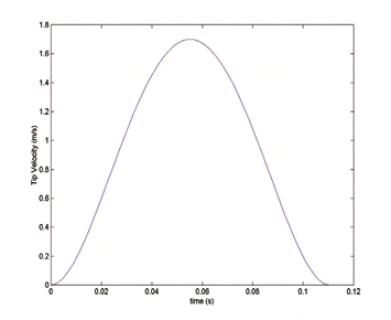
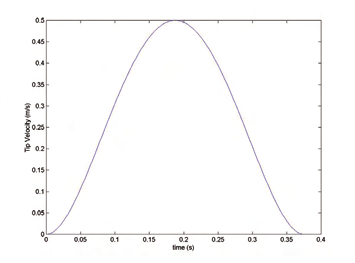
The first simulation is for high speed, with a maximum velocity of 102 m/min. The second
simulation is for low high speed with a maximum velocity of 30 m/min. In both cases, the
hexapod moves a distance of 0.1m along the z axis. The initial position of the moving
platform is at x o = 0, y o = 0 and z o = 0.7m. Figure 4 shows the velocity profiles of the moving
platform. Figures 5, 6 and 7 show the displacements, velocities and accelerations of the six
actuators, respectively. Figure 8 shows the computed actuator forces. The simulations show
that high speed motions result in large actuator forces.