Collaborative Statistics (MT230-Spring 2012) by Barbara Illowsky, Ph.D., Susan Dean - HTML preview

PLEASE NOTE: This is an HTML preview only and some elements such as links or page numbers may be incorrect.
Download the book in PDF, ePub, Kindle for a complete version.

Chapter 7The Central Limit Theorem

7.1The Central Limit Theorem*

This module provides a brief introduction to the Central Limit Theorem.

Student Learning Outcomes

By the end of this chapter, the student should be able to:

  • Recognize the Central Limit Theorem problems.

  • Classify continuous word problems by their distributions.

  • Apply and interpret the Central Limit Theorem for Means.

  • Apply and interpret the Central Limit Theorem for Sums.

Introduction

Why are we so concerned with means? Two reasons are that they give us a middle ground for comparison and they are easy to calculate. In this chapter, you will study means and the Central Limit Theorem.

The Central Limit Theorem (CLT for short) is one of the most powerful and useful ideas in all of statistics. Both alternatives are concerned with drawing finite samples of size n from a population with a known mean, μ , and a known standard deviation, σ . The first alternative says that if we collect samples of size n and n is "large enough," calculate each sample's mean, and create a histogram of those means, then the resulting histogram will tend to have an approximate normal bell shape. The second alternative says that if we again collect samples of size n that are "large enough," calculate the sum of each sample and create a histogram, then the resulting histogram will again tend to have a normal bell-shape.

In either case, it does not matter what the distribution of the original population is, or whether you even need to know it. The important fact is that the sample means and the sums tend to follow the normal distribution. And, the rest you will learn in this chapter.

The size of the sample, n, that is required in order to be to be 'large enough' depends on the original population from which the samples are drawn. If the original population is far from normal then more observations are needed for the sample means or the sample sums to be normal. Sampling is done with replacement.

Optional Collaborative Classroom Activity

Do the following example in class: Suppose 8 of you roll 1 fair die 10 times, 7 of you roll 2 fair dice 10 times, 9 of you roll 5 fair dice 10 times, and 11 of you roll 10 fair dice 10 times.

Each time a person rolls more than one die, he/she calculates the sample mean of the faces showing. For example, one person might roll 5 fair dice and get a 2, 2, 3, 4, 6 on one roll.

The mean is _autogen-svg2png-0007.png. _autogen-svg2png-0008.png The 3.4 is one mean when 5 fair dice are rolled. This same person would roll the 5 dice 9 more times and calculate 9 more means for a total of 10 means.

Your instructor will pass out the dice to several people as described above. Roll your dice 10 times. For each roll, record the faces and find the mean. Round to the nearest 0.5.

Your instructor (and possibly you) will produce one graph (it might be a histogram) for 1 die, one graph for 2 dice, one graph for 5 dice, and one graph for 10 dice. Since the "mean" when you roll one die, is just the face on the die, what distribution do these means appear to be representing?

Draw the graph for the means using 2 dice. Do the sample means show any kind of pattern?

Draw the graph for the means using 5 dice. Do you see any pattern emerging?

Finally, draw the graph for the means using 10 dice. Do you see any pattern to the graph? What can you conclude as you increase the number of dice?

As the number of dice rolled increases from 1 to 2 to 5 to 10, the following is happening:

  1. The mean of the sample means remains approximately the same.

  2. The spread of the sample means (the standard deviation of the sample means) gets smaller.

  3. The graph appears steeper and thinner.

You have just demonstrated the Central Limit Theorem (CLT).

The Central Limit Theorem tells you that as you increase the number of dice, the sample means tend toward a normal distribution (the sampling distribution).

7.2The Central Limit Theorem for Sample Means (Averages)*

Suppose X is a random variable with a distribution that may be known or unknown (it can be any distribution). Using a subscript that matches the random variable, suppose:

a. μX = the mean of X
b. σX = the standard deviation of X

If you draw random samples of size n, then as n increases, the random variable _autogen-svg2png-0008.png which consists of sample means, tends to be normally distributed and

_autogen-svg2png-0009.png ~ _autogen-svg2png-0010.png

The Central Limit Theorem for Sample Means says that if you keep drawing larger and larger samples (like rolling 1, 2, 5, and, finally, 10 dice) and calculating their means the sample means form their own normal distribution (the sampling distribution). The normal distribution has the same mean as the original distribution and a variance that equals the original variance divided by n, the sample size. n is the number of values that are averaged together not the number of times the experiment is done.

To put it more formally, if you draw random samples of size n,the distribution of the random variable _autogen-svg2png-0014.png, which consists of sample means, is called the sampling distribution of the mean. The sampling distribution of the mean approaches a normal distribution as n, the sample size, increases.

The random variable _autogen-svg2png-0016.png has a different z-score associated with it than the random variable X. _autogen-svg2png-0018.png is the value of _autogen-svg2png-0019.png in one sample.

(7.1)
_autogen-svg2png-0020.png

μX is both the average of X and of _autogen-svg2png-0023.png.

_autogen-svg2png-0024.png standard deviation of _autogen-svg2png-0025.png and is called the standard error of the mean.

Example 7.1

An unknown distribution has a mean of 90 and a standard deviation of 15. Samples of size n = 25 are drawn randomly from the population.

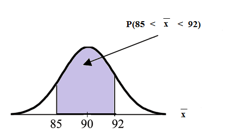
Find the probability that the sample mean is between 85 and 92.

Let X = one value from the original unknown population. The probability question asks you to find a probability for the sample mean.

Let _autogen-svg2png-0028.png the mean of a sample of size 25. Since μX = 90 , σX = 15 , and _autogen-svg2png-0031.png;

then _autogen-svg2png-0032.png ~ _autogen-svg2png-0033.png

Find _autogen-svg2png-0034.png Draw a graph.

_autogen-svg2png-0035.png

The probability that the sample mean is between 85 and 92 is 0.6997.

Normal distribution curve from -∞ to ∞ and an x-axis with the values of 85, 90, and 92. The x-axis is equal to the mean of a sample size of 25. A vertical upward line extends from points 85 and 92 to the curve. The probability area is between 85 and 92.

TI-83 or 84: normalcdf(lower value, upper value, mean, standard error of the mean)

The parameter list is abbreviated (lower value, upper value, μ, _autogen-svg2png-0037.png)

normalcdf_autogen-svg2png-0038.png

Find the value that is 2 standard deviations above the expected value (it is 90) of the sample mean.

To find the value that is 2 standard deviations above the expected value 90, use the formula

value = _autogen-svg2png-0039.png

value = _autogen-svg2png-0040.png

So, the value that is 2 standard deviations above the expected value is 96.

Example 7.2

The length of time, in hours, it takes an "over 40" group of people to play one soccer match is normally distributed with a mean of 2 hours and a standard deviation of 0.5 hours. A sample of size n = 50 is drawn randomly from the population.

Find the probability that the sample mean is between 1.8 hours and 2.3 hours.

Let X = the time, in hours, it takes to play one soccer match.

The probability question asks you to find a probability for the sample mean time, in hours, it takes to play one soccer match.

Let _autogen-svg2png-0043.png = the mean time, in hours, it takes to play one soccer match.

If μX = _________, σX = __________, and n= ___________, then _autogen-svg2png-0047.png by the Central Limit Theorem for Means.

μX = 2, σX = 0.5, n= 50, and _autogen-svg2png-0051.png

Find _autogen-svg2png-0052.png. _autogen-svg2png-0053.png Draw a graph.

_autogen-svg2png-0054.png

normalcdf_autogen-svg2png-0055.png

The probability that the mean time is between 1.8 hours and 2.3 hours is ______.

7.3The Central Limit Theorem for Sums*

Suppose X is a random variable with a distribution that may be known or unknown (it can be any distribution) and suppose:

a. μX = the mean of X
b. σX = the standard deviation of X

If you draw random samples of size n, then as n increases, the random variable ΣX which consists of sums tends to be normally distributed and

Σ X ~ _autogen-svg2png-0010.png

The Central Limit Theorem for Sums says that if you keep drawing larger and larger samples and taking their sums, the sums form their own normal distribution (the sampling distribution) which approaches a normal distribution as the sample size increases. The normal distribution has a mean equal to the original mean multiplied by the sample size and a standard deviation equal to the original standard deviation multiplied by the square root of the sample size.

The random variable Σ X has the following z-score associated with it:

a. Σx is one sum.
b. _autogen-svg2png-0013.png
a. nμX = the mean of ΣX
b. _autogen-svg2png-0016.png standard deviation of ΣX
Example 7.3

An unknown distribution has a mean of 90 and a standard deviation of 15. A sample of size 80 is drawn randomly from the population.

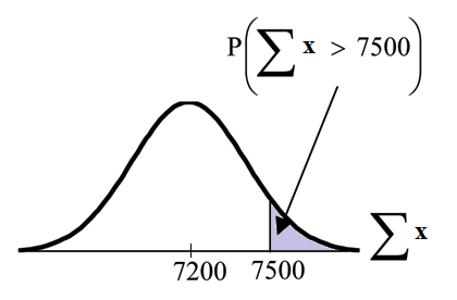
a. Find the probability that the sum of the 80 values (or the total of the 80 values) is more than 7500.
b. Find the sum that is 1.5 standard deviations above the mean of the sums.

Let X = one value from the original unknown population. The probability question asks you to find a probability for the sum (or total of) 80 values.

ΣX = the sum or total of 80 values. Since μX = 90 , σX = 15 , and n = 80 , then

Σ X ~ _autogen-svg2png-0024.png

  • mean of the sums = _autogen-svg2png-0025.png

  • standard deviation of the sums = _autogen-svg2png-0026.png

  • sum of 80 values = Σx = 7500

a: Find _autogen-svg2png-0028.png

P ( Σx > 7500 ) = 0.0127

Normal distribution curve of sum X with the values of 7200 and 7500 on the x-axis. A vertical upward line extends from point 7500 on the x-axis up to the curve. The probability area occurs from point 7500 and to the end of the curve.

normalcdf(lower value, upper value, mean of sums, stdev of sums)

The parameter list is abbreviated (lower, upper, _autogen-svg2png-0030.png)

normalcdf(7500,1E99, _aut			</div>
		</div>
		<div class=