A realizable filter must require only a finite number of
computations per output sample. For linear, causal, time-Invariant filters,
this restricts one to rational transfer functions of the form
 Assuming no pole-zero cancellations,
H(z)
is FIR if
ai=0 ,
i>0
, and IIR otherwise. Filter structures usually implement
rational transfer functions as difference equations.
Assuming no pole-zero cancellations,
H(z)
is FIR if
ai=0 ,
i>0
, and IIR otherwise. Filter structures usually implement
rational transfer functions as difference equations.
Whether FIR or IIR, a given transfer function can be implemented with many different filter structures. With infinite-precision data, coefficients, and arithmetic, all filter structures implementing the same transfer function produce the same output. However, different filter strucures may produce very different errors with quantized data and finite-precision or fixed-point arithmetic. The computational expense and memory usage may also differ greatly. Knowledge of different filter structures allows DSP engineers to trade off these factors to create the best implementation.
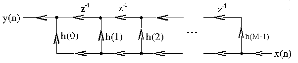
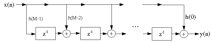
Consider causal FIR filters:
; this can be realized using the following structure
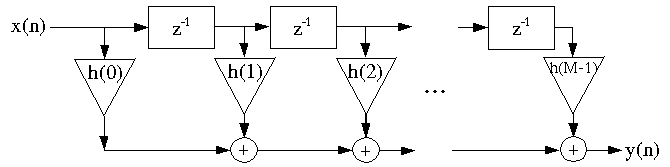
or in a different notation
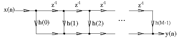
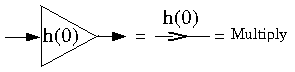
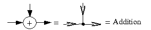
This is called the direct-form FIR filter structure.
There are no closed loops (no feedback) in this structure, so it is called a non-recursive structure. Since any FIR filter can be implemented using the direct-form, non-recursive structure, it is always possible to implement an FIR filter non-recursively. However, it is also possible to implement an FIR filter recursively, and for some special sets of FIR filter coefficients this is much more efficient.
 where
where
 But note that
y(n)=y(n−1)+x(n)−x(n−M)
This can be implemented as
But note that
y(n)=y(n−1)+x(n)−x(n−M)
This can be implemented as
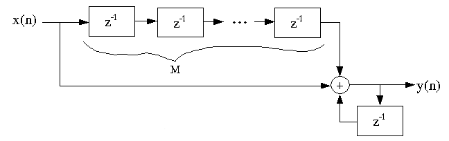
Instead of costing M−1 adds/output point, this comb filter costs only two adds/output.
Is this stable, and if not, how can it be made so?
IIR filters must be implemented with a recursive structure, since that's the only way a finite number of elements can generate an infinite-length impulse response in a linear, time-invariant (LTI) system. Recursive structures have the advantages of being able to implement IIR systems, and sometimes greater computational efficiency, but the disadvantages of possible instability, limit cycles, and other deletorious effects that we will study shortly.
The flow-graph-reversal theorem says that if one changes the directions of all the arrows, and inputs at the output and takes the output from the input of a reversed flow-graph, the new system has an identical input-output relationship to the original flow-graph.
The z-transform of an FIR filter can be factored into a
cascade of short-length filters
b0+b1z-1+b2z-3+…+bmz–m=b0(1−z1z-1)(1−z2z-1)…(1−zmz-1)
where the
zi are the zeros of this polynomial. Since the
coefficients of the polynomial are usually real, the roots
are usually complex-conjugate pairs, so we generally combine
 into one quadratic (length-2) section with
real coefficients
into one quadratic (length-2) section with
real coefficients
 The overall filter can then be implemented in a
cascade structure.
The overall filter can then be implemented in a
cascade structure.
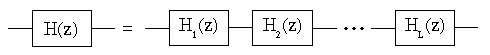
This is occasionally done in FIR filter implementation when one or more of the short-length filters can be implemented efficiently.
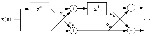
It is also possible to implement FIR filters in a lattice structure: this is sometimes used in adaptive filtering
IIR (Infinite Impulse Response) filter structures must be recursive
(use feedback); an infinite number of coefficients could not otherwise
be realized with a finite number of computations per sample.
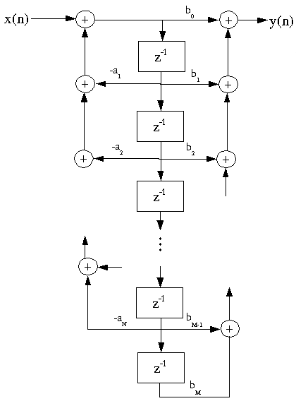
The corresponding time-domain difference equation is
y(n)=–(a1y(n−1))−a2y(n−2)+…−aNy(n−N)+b0x(0)+b1x(n−1)+…+bMx(n−M)
The difference equation above is implemented directly as written by the Direct-Form I IIR Filter Structure.
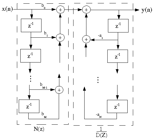
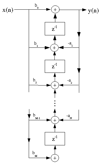
Note that this is a cascade of two systems,
N(z)
and
 . If we reverse the order of the filters, the overall
system is unchanged: The memory elements appear in the middle
and store identical values, so they can be combined, to form
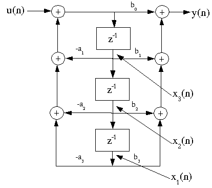
the Direct-Form II IIR Filter Structure.
. If we reverse the order of the filters, the overall
system is unchanged: The memory elements appear in the middle
and store identical values, so they can be combined, to form
the Direct-Form II IIR Filter Structure.
This structure is canonic: (i.e., it requires the minimum number of memory elements).
Flowgraph reversal gives the
Usually we design IIR filters with N=M , but not always.
Obviously, since all these structures have identical frequency response, filter structures are not unique. We consider many different structures because
The Cascade-Form IIR filter structure is one of the least sensitive to quantization, which is why it is the most commonly used IIR filter structure.
The numerator and denominator polynomials can be factored
 and implemented as a cascade of short IIR filters.
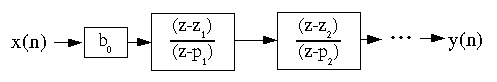
Since the filter coefficients are usually real yet the roots are mostly complex, we actually implement these as second-order sections, where comple-conjugate pole and zero pairs are combined into second-order sections with real coefficients. The second-order sections are usually implemented with either the Direct-Form II or Transpose-Form structure.
A rational transfer function can also be written as
 which by linearity can be implemented as
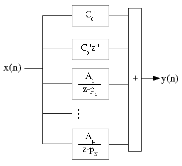
As before, we combine complex-conjugate pole pairs into second-order sections with real coefficients.
The cascade and parallel forms are of interest because they are much less sensitive to coefficient quantization than higher-order structures, as analyzed in later modules in this course.
There are many other structures for IIR filters, such as wave digital filter structures, lattice-ladder, all-pass-based forms, and so forth. These are the result of extensive research to find structures which are computationally efficient and insensitive to quantization error. They all represent various tradeoffs; the best choice in a given context is not yet fully understood, and may never be.
the minimum additional information at time n, which, along with all current and future input values, is necessary to compute all future outputs.
Essentially, the state of a system is the information held in the delay registers in a filter structure or signal flow graph.
Any LTI (linear, time-invariant) system of finite order M can be represented by a state-variable description x(n+1)=Ax(n)+Bu(n) y(n)=Cx(n)+Du(n) where x is an (M x 1) "state vector," u(n) is the input at time n, y(n) is the output at time n; A is an (M x M) matrix, B is an (M x 1) vector, C is a (1 x M) vector, and D is a (1 x 1) scalar.
One can always obtain a state-variable description of a signal flow graph.
y(n)=–(a1y(n−1))−a2y(n−2)−a3y(n−3)+b0x(n)+b1x(n−1)+b2x(n−2)+b3x(n−3)