Probability associates with an event a number which indicates the likelihood of the occurrence of that event on any trial. An event is modeled as the set of those possible outcomes of an experiment which satisfy a property or proposition characterizing the event.

Often, each outcome is characterized by a number. The experiment is performed. If the outcome is observed as a physical quantity, the size of that quantity (in prescribed units) is the entity actually observed. In many nonnumerical cases, it is convenient to assign a number to each outcome. For example, in a coin flipping experiment, a “head” may be represented by a 1 and a “tail” by a 0. In a Bernoulli trial, a success may be represented by a 1 and a failure by a 0. In a sequence of trials, we may be interested in the number of successes in a sequence of n component trials. One could assign a distinct number to each card in a deck of playing cards. Observations of the result of selecting a card could be recorded in terms of individual numbers. In each case, the associated number becomes a property of the outcome.

We consider in this chapter real random variables (i.e., real-valued random variables). In the chapter "Random Vectors and Joint Distributions", we extend the notion to vector-valued random quantites. The fundamental idea of a real random variable is the assignment of a real number to each elementary outcome ω in the basic space Ω. Such an assignment amounts to determining a function X, whose domain is Ω and whose range is a subset of the real line R. Recall that a real-valued function on a domain (say an interval I on the real line) is characterized by the assignment of a real number y to each element x (argument) in the domain. For a real-valued function of a real variable, it is often possible to write a formula or otherwise state a rule describing the assignment of the value to each argument. Except in special cases, we cannot write a formula for a random variable X. However, random variables share some important general properties of functions which play an essential role in determining their usefulness.

Mappings and inverse mappings

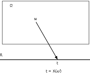
There are various ways of characterizing a function. Probably the most useful for our purposes is as a mapping from the domain Ω to the codomain R. We find the mapping diagram of Figure 1 extremely useful in visualizing the essential patterns. Random variable X, as a mapping from basic space Ω to the real line R, assigns to each element ω a value t=X(ω). The object point ω is mapped, or carried, into the image point t. Each ω is mapped into exactly one t, although several ω may have the same image point.

Figure 6.1. 

The basic mapping diagram .

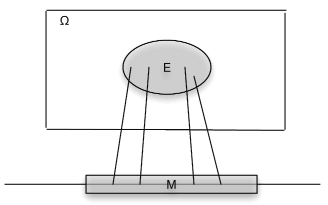
Associated with a function X as a mapping are the inverse mapping X^–1 and the inverse images it produces. Let M be a set of numbers on the real line. By the inverse image of M under the mapping X, we mean the set of all those ω∈Ω which are mapped into M by X (see Figure 2). If X does not take a value in M, the inverse image is the empty set (impossible event). If M includes the range of X, (the set of all possible values of X), the inverse image is the entire basic space Ω. Formally we write

(6.1)

Now we assume the set X^–1(M), a subset of Ω, is an event for each M. A detailed examination of that assertion is a topic in measure theory. Fortunately, the results of measure theory ensure that we may make the assumption for any X and any subset M of the real line likely to be encountered in practice. The set X^–1(M) is the event that X takes a value in M. As an event, it may be assigned a probability.

Figure 6.2. 

E is the inverse image X^–1(M).

Before considering further examples, we note a general property of inverse images. We state it in terms of a random variable, which maps Ω to the real line (see Figure 3).

Preservation of set operations

Let X be a mapping from Ω to the real line R. If M,M_i,i∈J, are sets of real numbers, with respective inverse images E,E_i, then

(6.4)

Examination of simple graphical examples exhibits the plausibility of these patterns. Formal proofs amount to careful reading of the notation. Central to the structure are the facts that each element ω is mapped into only one image point t and that the inverse image of M is the set of all those ω which are mapped into image points in M.

Figure 6.3. 

Preservation of set operations by inverse images.

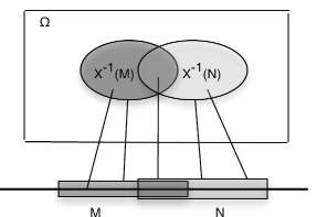
An easy, but important, consequence of the general patterns is that the inverse images of disjoint M,N are also disjoint. This implies that the inverse of a disjoint union of M_i is a disjoint union of the separate inverse images.

Example 6.2.  Events determined by a random variable

Consider, again, the random variable S_n which counts the number of successes in a sequence of n Bernoulli trials. Let n=10 and p=0.33. Suppose we want to determine the probability . Let , which we usually shorten to . Now the A_k form a partition, since we cannot have ω∈A_k and (i.e., for any ω, we cannot have two values for S_n(ω)). Now,

(6.5)

since S₁₀ takes on a value greater than 2 but no greater than 8 iff it takes one of the integer values from 3 to 8. By the additivity of probability,

(6.6)

Because of the abstract nature of the basic space and the class of events, we are limited in the kinds of calculations that can be performed meaningfully with the probabilities on the basic space. We represent probability as mass distributed on the basic space and visualize this with the aid of general Venn diagrams and minterm maps. We now think of the mapping from Ω to R as a producing a point-by-point transfer of the probability mass to the real line. This may be done as follows:

To any set M on the real line assign probability mass

It is apparent that P_X(M)≥0 and P_X(R)=P(Ω)=1. And because of the preservation of set operations by the inverse mapping

(6.7)

This means that P_X has the properties of a probability measure defined on the subsets of the real line. Some results of measure theory show that this probability is defined uniquely on a class of subsets of R that includes any set normally encountered in applications. We have achieved a point-by-point transfer of the probability apparatus to the real line in such a manner that we can make calculations about the random variable X. We call P_X the probability measure induced byX. Its importance lies in the fact that P(X∈M)=P_X(M). Thus, to determine the likelihood that random quantity X will take on a value in set M, we determine how much induced probability mass is in the set M. This transfer produces what is called the probability distribution for X. In the chapter "Distribution and Density Functions", we consider useful ways to describe the probability distribution induced by a random variable. We turn first to a special class of random variables.

We consider, in some detail, random variables which have only a finite set of possible values. These are called simple random variables. Thus the term “simple” is used in a special, technical sense. The importance of simple random variables rests on two facts. For one thing, in practice we can distinguish only a finite set of possible values for any random variable. In addition, any random variable may be approximated as closely as pleased by a simple random variable. When the structure and properties of simple random variables have been examined, we turn to more general cases. Many properties of simple random variables extend to the general case via the approximation procedure.

Representation with the aid of indicator functions

In order to deal with simple random variables clearly and precisely, we must find suitable ways to express them analytically. We do this with the aid of indicator functions. Three basic forms of representation are encountered. These are not mutually exclusive representatons.