In the unit on Random Variables and Probability we introduce real random variables as mappings from the basic space Ω to the real line. The mapping induces a transfer of the probability mass on the basic space to subsets of the real line in such a way that the probability that X takes a value in a set M is exactly the mass assigned to that set by the transfer. To perform probability calculations, we need to describe analytically the distribution on the line. For simple random variables this is easy. We have at each possible value of X a point mass equal to the probability X takes that value. For more general cases, we need a more useful description than that provided by the induced probability measure PX.
In the theoretical discussion on Random Variables and Probability, we note that the probability distribution induced by a random variable X is determined uniquely by a consistent assignment of mass to semi-infinite intervals of the form (–∞,t] for each real t. This suggests that a natural description is provided by the following.
Definition
The distribution function FX for random variable X is given by

In terms of the mass distribution on the line, this is the probability mass at or to the left of the point t. As a consequence, FX has the following properties:
| (F1) : FX must be a nondecreasing function, for if t>s there must be at least as much probability mass at or to the left of t as there is for s. |
(F2) : FX is continuous from the right, with a jump in the amount p0 at
t0 iff
 . If the point t approaches t0 from the left, the interval
does not include the probability mass at t0 until t reaches that value, at which point the
amount at or to the left of t increases ("jumps") by amount p0; on the other hand, if t approaches t0
from the right, the interval includes the mass p0 all the way to and including t0, but drops
immediately as t moves to the left of t0. . If the point t approaches t0 from the left, the interval
does not include the probability mass at t0 until t reaches that value, at which point the
amount at or to the left of t increases ("jumps") by amount p0; on the other hand, if t approaches t0
from the right, the interval includes the mass p0 all the way to and including t0, but drops
immediately as t moves to the left of t0.
|
(F3) : Except in very unusual cases involving random variables which may take “infinite”
values, the probability mass included in  must increase to one as
t moves to the right; as t moves to the left, the probability mass included must decrease
to zero, so that must increase to one as
t moves to the right; as t moves to the left, the probability mass included must decrease
to zero, so that
(7.2)  |
A distribution function determines the probability mass in each semiinfinite interval (–∞,t]. According to the discussion referred to above, this determines uniquely the induced distribution.
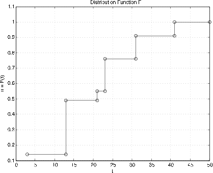
The distribution function FX for a simple random variable is easily visualized. The distribution consists of point mass pi at each point ti in the range. To the left of the smallest value in the range, FX(t)=0; as t increases to the smallest value t1, FX(t) remains constant at zero until it jumps by the amount p1.. FX(t) remains constant at p1 until t increases to t2, where it jumps by an amount p2 to the value p1+p2. This continues until the value of FX(t)reaches 1 at the largest value tn. The graph of FX is thus a step function, continuous from the right, with a jump in the amount pi at the corresponding point ti in the range. A similar situation exists for a discrete-valued random variable which may take on an infinity of values (e.g., the geometric distribution or the Poisson distribution considered below). In this case, there is always some probability at points to the right of any ti, but this must become vanishingly small as t increases, since the total probability mass is one.
The procedure ddbn may be used to plot the distributon function for a simple random variable from a matrix X of values and a corresponding matrix PX of probabilities.
>> c = [10 18 10 3];             % Distribution for X in Example 6.5.1
>> pm = minprob(0.1*[6 3 5]);
>> canonic
 Enter row vector of coefficients  c
 Enter row vector of minterm probabilities  pm
Use row matrices X and PX for calculations
Call for XDBN to view the distribution
>> ddbn                          % Circles show values at jumps
Enter row matrix of VALUES  X
Enter row matrix of PROBABILITIES  PX
%  Printing details   See Figure 7.1
We make repeated use of a number of common distributions which are used in many practical situations. This collection includes several distributions which are studied in the chapter "Random Variables and Probabilities".
Indicator function. X=IE P(X=1)=P(E)=pP(X=0)=q=1–p. The distribution function has a jump in the amount q at t=0 and an additional jump of p to the value 1 at t=1.
Simple random variable  (canonical form)

The distribution function is a step function, continuous from the right, with jump of pi at t=ti (See Figure 7.1 for Example 7.1)
Binomial (n,p). This random variable appears as the number of successes in a sequence of n Bernoulli trials with probability p of success. In its simplest form


As pointed out in the study of Bernoulli sequences in the unit on Composite Trials, two m-functions ibinom andcbinom are available for computing the individual and cumulative binomial probabilities.
Geometric (p) There are two related distributions, both arising in the study of continuing Bernoulli sequences. The first counts the number of failures before the first success. This is sometimes called the “waiting time.” The event {X=k} consists of a sequence of k failures, then a success. Thus

The second designates the component trial on which the first success occurs. The event {Y=k} consists of k–1 failures, then a success on the kth component trial. We have

We say X has the geometric distribution with parameter (p), which we often designate by X∼ geometric (p). Now Y=X+1 or Y–1=X. For this reason, it is customary to refer to the distribution for the number of the trial for the first success by saying Y–1∼ geometric (p). The probability of k or more failures before the first success is P(X≥k)=qk. Also

This suggests that a Bernoulli sequence essentially "starts over" on each trial. If it has failed n times, the probability of failing an additional k or more times before the next success is the same as the initial probability of failing k or more times before the first success.
A statistician is taking a random sample from a population in which two percent of the members own a BMW automobile. She takes a sample of size 100. What is the probability of finding no BMW owners in the sample?
The sampling process may be viewed as a sequence of Bernoulli trials with probability p=0.02 of success. The probability of 100 or more failures before the first success is 0.98100=0.1326 or about 1/7.5.
Negative binomial (m,p). X is the number of failures before the mth success. It is generally more convenient to work with Y=X+m, the number of the trial on which the mth success occurs. An examination of the possible patterns and elementary combinatorics show that

There are m–1 successes in the first k–1 trials, then a success. Each combination has probability pmqk–m. We have an m-function nbinom to calculate these probabilities.
A player throws a single six-sided die repeatedly. He scores if he throws a 1 or a 6. What is the probability he scores five times in ten or fewer throws?
>> p = sum(nbinom(5,1/3,5:10))
p  =  0.2131
An alternate solution is possible with the use of the binomial distribution. The mth success comes not later than the kth trial iff the number of successes in k trials is greater than or equal to m.
>> P = cbinom(10,1/3,5)
P  =  0.2131
Poisson (μ). This distribution is assumed in a wide variety of applications. It appears as a counting variable for items arriving with exponential interarrival times (see the relationship to the gamma distribution below). For large n and small p (which may not be a value found in a table), the binomial distribution is approximately Poisson (np). Use of the generating function (see Transform Methods) shows the sum of independent Poisson random variables is Poisson. The Poisson distribution is integer valued, with

Although Poisson probabilities are usually easier to calculate with scientific calculators than binomial probabilities, the use of tables is often quite helpful. As in the case of the binomial distribution, we have two m-functions for calculating Poisson probabilities. These have advantages of speed and parameter range similar to those for ibinom and cbinom.
: P(X=k) is calculated by P = ipoisson(mu,k), where k is a row or
column vector of integers and the result P is a row matrix of the probabilities.
|
: P(X≥k) is calculated by P = cpoisson(mu,k), where k is a row
or column vector of integers and the result P is a row matrix of the probabilities.
|
The number of messages arriving in a one minute period at a communications network junction is a random variable N∼ Poisson (130). What is the probability the number of arrivals is greater than equal to 110, 120, 130, 140, 150, 160 ?
>> p = cpoisson(130,110:10:160)
p  =  0.9666  0.8209  0.5117  0.2011  0.0461  0.0060
The descriptions of these distributions, along with a number of other facts, are summarized in the table DATA ON SOME COMMON DISTRIBUTIONS in Appendix C.
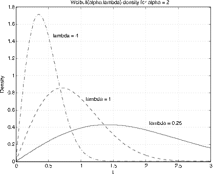
If the probability mass in the induced distribution is spread smoothly along the real line, with no point mass concentrations, there is a probability density function fX which satisfies

At each t, fX(t) is the mass per unit length in the probability distribution. The density function has three characteristic properties:

A random variable (or distribution) which has a density is called absolutely continuous. This term comes from measure theory. We often simply abbreviate as continuous distribution.
There is a technical mathematical description of the condition “spread smoothly with no point mass concentrations.” And strictly speaking the integrals are Lebesgue integrals rather than the ordinary Riemann kind. But for practical cases, the two agree, so that we are free to use ordinary integration techniques.
By the fundamental theorem of calculus

Any integrable, nonnegative function f with ∫f=1 determines a distribution function F , which in turn determines a probability distribution. If ∫f≠1, multiplication by the appropriate positive constant gives a suitable f . An argument based on the Quantile Function shows the existence of a random variable with that distribution.
In the literature on probability, it is customary to omit the indication of the region of integration when integrating over the whole line. Thus

The first expression is not an indefinite integral. In many situations, fX will be zero outside an interval. Thus, the integrand effectively determines the region of integration.