The concept of independence for classes of events is developed in terms of a product rule. In this unit, we extend the concept to classes of random variables.
Recall that for a random variable X, the inverse image X–1(M) (i.e., the set of all outcomes ω∈Ω which are mapped into M by X) is an event for each reasonable subset M on the real line. Similarly, the inverse image Y–1(N) is an event determined by random variable Y for each reasonable set N. We extend the notion of independence to a pair of random variables by requiring independence of the events they determine. More precisely,
Definition
A pair {X,Y} of random variables is (stochastically) independent
iff each pair of events  is independent.
This condition may be stated in terms of the product rule

Independence implies


Note that the product rule on the distribution function is equivalent to the condition the product rule holds for the inverse images of a special class of sets {M,N} of the form M=(–∞,t] and N=(–∞,u]. An important theorem from measure theory ensures that if the product rule holds for this special class it holds for the general class of {M,N}. Thus we may assert
The pair  is independent iff the following product rule holds

Suppose  . Taking limits shows

so that the product rule  holds. The pair
  is
therefore independent.
is
therefore independent.
If there is a joint density function, then the relationship to the joint distribution function makes it clear that the pair is independent iff the product rule holds for the density. That is, the pair is independent iff

Suppose the joint probability mass distributions induced by the pair  is
uniform on a rectangle with sides
is
uniform on a rectangle with sides  and
and  . Since the area
is (b–a)(d–c), the constant value of fXY is 1/(b–a)(d–c). Simple integration gives
. Since the area
is (b–a)(d–c), the constant value of fXY is 1/(b–a)(d–c). Simple integration gives


Thus it follows that X is uniform on  , Y is uniform on
  , and
, and
 for all t,u, so that the pair
 is independent. The converse is also true: if the pair is independent with
X uniform on
is independent. The converse is also true: if the pair is independent with
X uniform on  and Y is uniform on
  , the the pair has uniform joint
distribution on I1×I2.
, the the pair has uniform joint
distribution on I1×I2.
It should be apparent that the independence condition puts restrictions on the character of the joint mass distribution on the plane. In order to describe this more succinctly, we employ the following terminology.
Definition
If M is a subset of the horizontal axis and N is a subset of the vertical axis,
then the cartesian product M×N is the (generalized) rectangle consisting of
those points  on the plane such that t∈M and u∈N.
The rectangle in Example 9.2 is the Cartesian product I1×I2, consisting of all those
points  such that a≤t≤b and c≤u≤d (i.e., t∈I1
and u∈I2).
such that a≤t≤b and c≤u≤d (i.e., t∈I1
and u∈I2).
We restate the product rule for independence in terms of cartesian product sets.

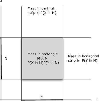
Reference to Figure 9.1 illustrates the basic pattern. If M, N are intervals on the horizontal and vertical axes, respectively, then the rectangle M×N is the intersection of the vertical strip meeting the horizontal axis in M with the horizontal strip meeting the vertical axis in N. The probability X∈M is the portion of the joint probability mass in the vertical strip; the probability Y∈N is the part of the joint probability in the horizontal strip. The probability in the rectangle is the product of these marginal probabilities.
This suggests a useful test for nonindependence which we call the rectangle test. We illustrate with a simple example.
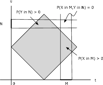
Supose probability mass is uniformly distributed over the square with vertices at (1,0), (2,1), (1,2), (0,1). It is evident from Figure 9.2 that a value of X determines the possible values of Y and vice versa, so that we would not expect independence of the pair. To establish this, consider the small rectangle M×N shown on the figure. There is no probability mass in the region. Yet P(X∈M)>0 and P(Y∈N)>0, so that
 , but
, but
 . The product rule fails; hence
the pair cannot be stochastically independent.
. The product rule fails; hence
the pair cannot be stochastically independent.
Remark. There are nonindependent cases for which this test does not work. And it does not provide a test for independence. In spite of these limitations, it is frequently useful. Because of the information contained in the independence condition, in many cases the complete joint and marginal distributions may be obtained with appropriate partial information. The following is a simple example.
Suppose the pair  is independent and each has three possible values. The
following four items of information are available.
is independent and each has three possible values. The
following four items of information are available.


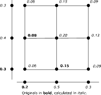
These values are shown in bold type on Figure 9.3. A combination of the product rule
and the fact that the total probability mass is one are used to calculate each of
the marginal and joint probabilities. For example  and
and

 implies
  . Then
 . Others are calculated
similarly. There is no unique procedure for solution. And it has not seemed
useful to develop MATLAB procedures to accomplish this.
. Others are calculated
similarly. There is no unique procedure for solution. And it has not seemed
useful to develop MATLAB procedures to accomplish this.
A pair  has the joint normal distribution iff the joint density is

where

The marginal densities are obtained with the aid of some algebraic tricks to integrate
the joint density. The result is that  and
and  . If the parameter ρ is set to zero, the result is

so that the pair is independent iff ρ=0. The details are left as an exercise for the interested reader.
Remark. While it is true that every independent pair of normally distributed random variables is joint normal, not every pair of normally distributed random variables has the joint normal distribution.
We start with the distribution for a joint normal pair and derive a joint distribution for a normal pair which is not joint normal. The function

is the joint normal density for an independent pair (ρ=0) of standardized normal
random variables. Now define the joint density for a pair  by
by

Both  and
and  . However, they cannot be joint normal, since the joint
normal distribution is positive for all
. However, they cannot be joint normal, since the joint
normal distribution is positive for all  .
.
Since independence of random variables is independence of the events determined by the random variables, extension to general classes is simple and immediate.
Definition
A class  of random variables is (stochastically)
independent iff the product rule holds for
every finite subclass of two or more.
of random variables is (stochastically)
independent iff the product rule holds for
every finite subclass of two or more.
Remark. The index set J in the definition may be finite or infinite.
For a finite class  , independence is equivalent to the product
rule
, independence is equivalent to the product
rule

Since we may obtain the joint distribution function for any finite subclass by letting the arguments for the others be ∞ (i.e., by taking the limits as the appropriate ti increase without bound), the single product rule suffices to account for all finite subclasses.
Absolutely continuous random variables
If a class  is independent and the individual variables are absolutely
continuous (i.e., have densities), then any finite subclass is jointly absolutely
continuous and the product rule holds for the densities of such subclasses
is independent and the individual variables are absolutely
continuous (i.e., have densities), then any finite subclass is jointly absolutely
continuous and the product rule holds for the densities of such subclasses

Similarly, if each finite subclass is jointly absolutely continuous, then each individual variable is absolutely continuous and the product rule holds for the densities. Frequently we deal with independent classes in which each random variable has the same marginal distribution. Such classes are referred to as iid classes (an acronym for independent,identically distributed). Examples are simple random samples from a given population, or the results of repetitive trials with the same distribution on the outcome of each component trial. A Bernoulli sequence is a simple example.
Consider a pair  of simple random variables in canonical form

Since