The probability that real random variable X takes a value in a set M of real numbers is interpreted as the likelihood that the observed value X(ω) on any trial will lie in M. Historically, this idea of likelihood is rooted in the intuitive notion that if the experiment is repeated enough times the probability is approximately the fraction of times the value of X will fall in M. Associated with this interpretation is the notion of the average of the values taken on. We incorporate the concept of mathematical expectation into the mathematical model as an appropriate form of such averages. We begin by studying the mathematical expectation of simple random variables, then extend the definition and properties to the general case. In the process, we note the relationship of mathematical expectation to the Lebesque integral, which is developed in abstract measure theory. Although we do not develop this theory, which lies beyond the scope of this study, identification of this relationship provides access to a rich and powerful set of properties which have far reaching consequences in both application and theory.

The notion of mathematical expectation is closely related to the idea of a weighted mean, used extensively in the handling of numerical data. Consider the arithmetic average of the following ten numbers: 1, 2, 2, 2, 4, 5, 5, 8, 8, 8, which is given by

(11.1)

Examination of the ten numbers to be added shows that five distinct values are included. One of the ten, or the fraction 1/10 of them, has the value 1, three of the ten, or the fraction 3/10 of them, have the value 2, 1/10 has the value 4, 2/10 have the value 5, and 3/10 have the value 8. Thus, we could write

(11.2)

The pattern in this last expression can be stated in words: Multiply each possible value by the fraction of the numbers having that value and then sum these products. The fractions are often referred to as the relative frequencies. A sum of this sort is known as a weighted average.

In general, suppose there are n numbers to be averaged, with m≤n distinct values . Suppose f₁ have value t₁, f₂ have value have value t_m. The f_i must add to n. If we set p_i=f_i/n, then the fraction p_i is called the relative frequency of those numbers in the set which have the value t_i,1≤i≤m. The average of the n numbers may be written

(11.3)

In probability theory, we have a similar averaging process in which the relative frequencies of the various possible values of are replaced by the probabilities that those values are observed on any trial.

Definition. For a simple random variable X with values and corresponding probabilities , the mathematical expectation, designated E[X], is the probability weighted average of the values taken on by X. In symbols

(11.4)

Note that the expectation is determined by the distribution. Two quite different random variables may have the same distribution, hence the same expectation. Traditionally, this average has been called the mean, or the mean value, of the random variable X.

Figure 11.1. 

Moment of a probability distribution about the origin.

Mechanical interpretation

In order to aid in visualizing an essentially abstract system, we have employed the notion of probability as mass. The distribution induced by a real random variable on the line is visualized as a unit of probability mass actually distributed along the line. We utilize the mass distribution to give an important and helpful mechanical interpretation of the expectation or mean value. In Example 6 in "Mathematical Expectation: General Random Variables", we give an alternate interpretation in terms of mean-square estimation.

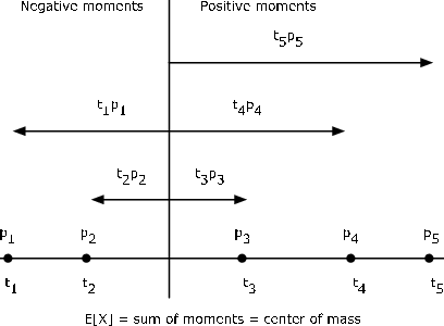
Suppose the random variable X has values , with . This produces a probability mass distribution, as shown in Figure 1, with point mass concentration in the amount of p_i at the point t_i. The expectation is

(11.6)

Now |t_i| is the distance of point mass p_i from the origin, with p_i to the left of the origin iff t_i is negative. Mechanically, the sum of the products t_ip_i is the moment of the probability mass distribution about the origin on the real line. From physical theory, this moment is known to be the same as the product of the total mass times the number which locates the center of mass. Since the total mass is one, the mean value is the location of the center of mass. If the real line is viewed as a stiff, weightless rod with point mass p_i attached at each value t_i of X, then the mean value μ_X is the point of balance. Often there are symmetries in the distribution which make it possible to determine the expectation without detailed calculation.

Example 11.2. The number of spots on a die

Let X be the number of spots which turn up on a throw of a simple six-sided die. We suppose each number is equally likely. Thus the values are the integers one through six, and each probability is 1/6. By definition

(11.7)

Although the calculation is very simple in this case, it is really not necessary. The probability distribution places equal mass at each of the integer values one through six. The center of mass is at the midpoint.

For a simple random variable, the mathematical expectation is determined as the dot product of the value matrix with the probability matrix. This is easily calculated using MATLAB.

X = [2 2.5 3 3.5];  % Matrix of values (ordered)
PX = 0.1*[2 2 3 3]; % Matrix of probabilities
EX = dot(X,PX)      % The usual MATLAB operation
EX =  2.8500
Ex = sum(X.*PX)     % An alternate calculation
Ex =  2.8500
ex = X*PX'          % Another alternate
ex =  2.8500

Expectation and primitive form

The definition and treatment above assumes X is in canonical form, in which case

(11.9)

We wish to ease this restriction to canonical form.

Suppose simple random variable X is in a primitive form

(11.10)

We show that

(11.11)

Before a formal verification, we begin with an example which exhibits the essential pattern. Establishing the general case is simply a matter of appropriate use of notation.

Example 11.5. Simple random variable X in primitive form

(11.12)

Inspection shows the distinct possible values of X to be 1, 2, or 3. Also,

(11.13)

so that

(11.14)

Now

(11.15)

(11.16)

To establish the general pattern, consider . We identify the distinct set of values contained in the set . Suppose these are t₁<t₂<⋯<t_n. For any value t_i in the range, identify the index set J_i of those j such that c_j=t_i. Then the terms

(11.17)

By the additivity of probability

(11.18)

Since for each j∈J_i we have c_j=t_i, we have

(11.19)

— □

Thus, the defining expression for expectation thus holds for X in a primitive form.

An alternate approach to obtaining the expectation from a primitive form is to use the csort operation to determine the distribution of X from the coefficients and probabilities of the primitive form.

Example 11.6. Alternate determinations of E[X]

Suppose X in a primitive form is

(11.20) X = I_C1 + 2 I_C2 + I_C3 + 3 I_C4 + 2 I_C5 + 2 I_C6 + I_C7 + 3 I_C8 + 2 I_C9 + I_C10

with respective probabilities

(11.21)

c = [1 2 1 3 2 2 1 3 2 1];            % Matrix of coefficients
pc = 0.01*[8 11 6 13 5 8 12 7 14 16]; % Matrix of probabilities
EX = c*pc'
EX =   1.7800                         % Direct solution
[X,PX] = csort(c,pc);                 % Determination of dbn for X
disp([X;PX]')
    1.0000    0.4200
    2.0000    0.3800
    3.0000    0.2000
Ex = X*PX'                            %  E[X] from distribution
Ex =   1.7800

Linearity

The result on primitive forms may be used to establish the linearity of mathematical expectation for simple random variables. Because of its fundamental importance, we work through the verification in some detail.

Suppose and (both in canonical form). Since

(11.22)

we have

(11.23)

Note that I_AiI_Bj=I_AiBj and . The class of these sets for all possible pairs forms a partition. Thus, the last summation expresses Z=X+Y in a primitive form. Because of the result on primitive forms, above, we have

(11.24)

(11.25)

We note that for each i and for each j

(11.26)

Hence, we may write

(11.27)

Page 1Page 2Page 3Page 4Page 5Page 6Page 7Page 8Page 9Page 10Page 11Page 12Page 13Page 14Page 15Page 16Page 17Page 18Page 19Page 20Page 21Page 22Page 23Page 24Page 25

PREV   NEXT