The definition of conditional independence of events is based on a product rule which may be expressed in terms of conditional expectation, given an event. The pair is conditionally independent, given C, iff

(16.1)

If we let A=X^–1(M) and B=Y^–1(N), then I_A=I_M(X) and I_B=I_N(Y). It would be reasonable to consider the pair conditionally independent, given event C, iff the product rule

(16.2)

holds for all reasonable M and N (technically, all Borel M and N). This suggests a possible extension to conditional expectation, given a random vector. We examine the following concept.

Definition. The pair {X,Y} is conditionally independent, givenZ, designated , iff

(16.3)

Remark. Since it is not necessary that , or Z be real valued, we understand that the sets M and N are on the codomains for X and Y, respectively. For example, if X is a three dimensional random vector, then M is a subset of R³.

As in the case of other concepts, it is useful to identify some key properties, which we refer to by the numbers used in the table in Appendix G. We note two kinds of equivalences. For example, the following are equivalent.

(CI1)

(CI5)

Because the indicator functions are special Borel functions, (CI1) is a special case of (CI5). To show that (CI1) implies (CI5), we need to use linearity, monotonicity, and monotone convergence in a manner similar to that used in extending properties (CE1) to (CE6) for conditional expectation. A second kind of equivalence involves various patterns. The properties (CI1), (CI2), (CI3), and (CI4) are equivalent, with (CI1) being the defining condition for .

(CI1)

(CI2)

(CI3)

(CI4)

As an example of the kinds of argument needed to verify these equivalences, we show the equivalence of (CI1) and (CI2).

Use of property (CE8) shows that (CI2) and (CI3) are equivalent. Now just as (CI1) extends to (CI5), so also (CI3) is equivalent to

(CI6)

Property (CI6) provides an important interpretation of conditional independence:

is the best mean-square estimator for , given knowledge of Z. The condition implies that additional knowledge about Y does not modify that best estimate. This interpretation is often the most useful as a modeling assumption.

Similarly, property (CI4) is equivalent to

(CI8)

Property (CI7) is an alternate way of expressing (CI6). Property (CI9) is just a convenient way of expressing the other conditions.

The additional properties in Appendix G are useful in a variety of contexts, particularly in establishing properties of Markov systems. We refer to them as needed.

In the classical approach to statistics, a fundamental problem is to obtain information about the population distribution from the distribution in a simple random sample. There is an inherent difficulty with this approach. Suppose it is desired to determine the population mean μ. Now μ is an unknown quantity about which there is uncertainty. However, since it is a constant, we cannot assign a probability such as P(a<μ≤b). This has no meaning.

The Bayesian approach makes a fundamental change of viewpoint. Since the population mean is a quantity about which there is uncertainty, it is modeled as a random variable whose value is to be determined by experiment. In this view, the population distribution is conceived as randomly selected from a class of such distributions. One way of expressing this idea is to refer to a state of nature. The population distribution has been “selected by nature” from a class of distributions. The mean value is thus a random variable whose value is determined by this selection. To implement this point of view, we assume

The Bayesian model

If X is a random variable whose distribution is the population distribution and H is the parameter random variable, then have a joint distribution.

Population proportion

We illustrate these ideas with one of the simplest, but most important, statistical problems: that of determining the proportion of a population which has a particular characteristic. Examples abound. We mention only a few to indicate the importance.

The parameter in this case is the proportion p who meet the criterion. If sampling is at random, then the sampling process is equivalent to a sequence of Bernoulli trials. If H is the parameter random variable and S_n is the number of “successes” in a sample of size n, then the conditional distribution for S_n, given H=u, is binomial . To see this, consider

(16.14)

Anaysis is carried out for each fixed u as in the ordinary Bernoulli case. If

(16.15)

we have the result

(16.16)

The objective

We seek to determine the best mean-square estimate of H, given S_n=k. Two steps must be taken:

The Bayesian reversal

Since is an event with positive probability, we use the definition of the conditional expectation, given an event, and the law of total probability (CE1b) to obtain

(16.17)

(16.18)

A prior distribution for H

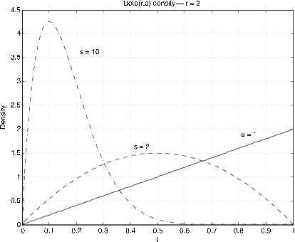
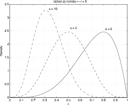
The beta distribution (see Appendix G), proves to be a “natural” choice for this purpose. Its range is the unit interval, and by proper choice of parameters the density function can be given a variety of forms (see Figures 1 and 2).

Figure 16.1. 

The Beta(r,s) density for .

Figure 16.2. 

The Beta(r,s) density for .

Its analysis is based on the integrals

(16.19)

For H∼ beta , the density is given by

(16.20)

For , f_H has a maximum at (r–1)/(r+s–2). For positive integers, f_H is a polynomial on , so that determination of the distribution function is easy. In any case, straightforward integration, using the integral formula above, shows

(16.21)

If the prior distribution for H is beta we may complete the determination of as follows.

(16.22)

(16.23)

We may adapt the analysis above to show that H is conditionally beta