To explain Rader's conversion of a prime p point DFT into a p–1 point circular convolution 1 we recall the definition of the DFT

(4.1)

with W = exp – j 2 π / p . Also recall that a primitive root of p is an integer r such that maps the integers m = 0 , ⋯ , p – 2 to the integers 1 , ⋯ , p – 1 . Letting n = r ^{– m} and k = r^l, where r ^{– m} is the inverse of r^m modulo p , the DFT becomes

(4.2)

for l=0,⋯,p–2. The `DC' term fis given by By defining new functions

(4.3)

which are simply permuted versions of the original sequences, the DFT becomes

(4.4)

for l=0,⋯,p–2. This equation describes circular convolution and therefore any circular convolution algorithm can be used to compute a prime length DFT. It is only necessary to (i) permute the input, the roots of unity and the output, (ii) add x(0) to each term in Equation 4.4 and (iii) compute the DC term.

To describe a bilinear form for the DFT we first define a permutation matrix Q for the permutation above. If p is a prime and r is a primitive root of p, then let Q_r be the permutation matrix defined by

(4.5)

for 0≤k≤p–2 where e_k is the k^th standard basis vector. Let the be a p–1 point vector of the roots of unity:

(4.6)

If s is the inverse of r modulo p (that is, rs=1 modulo p) and , then the circular convolution of Equation 4.4 can be computed with the bilinear form of ???:

(4.7)

This bilinear form does not compute y(0), the DC term. Furthermore, it is still necessary to add the x(0) term to each of the elements of Equation 4.7 to obtain y(1),⋯,y(p–1).

The computation of y(0) turns out to be very simple when the bilinear form Equation 4.7 is used to compute the circular convolution in Equation 4.4. The first element of in Equation 4.7 is the residue modulo the polynomial s–1, that is, the first element of this vector is the sum of the elements of . (The first row of the matrix, R, representing the reduction operation is a row of 1's, and the matrices P and Q_r are permutation matrices.) Therefore, the DC term can be computed by adding the first element of to x(0). Hence, when the Winograd or split nesting algorithm is used to perform the circular convolution of Equation 4.7, the computation of the DC term requires only one extra complex addition for complex data.

The addition x(0) to each of the elements of Equation 4.7 also requires only one complex addition. By adding x(0) to the first element of in Equation 4.7 and applying Q_s^tJP^tR^t to the result, x(0) is added to each element. (Again, this is because the first column of R^t is a column of 1's, and the matrices Q_s^t, J and P^t are permutation matrices.)

Although the DFT can be computed by making these two extra additions, this organization of additions does not yield a bilinear form. However, by making a minor modification, a bilinear form can be retrieved. The method described above can be illustrated in Figure 4.1 with .

Figure 4.1. 

The flow graph for the computation of the DFT.

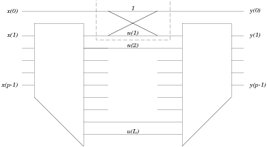
Clearly, the structure highlighted in the dashed box can be replaced by the structure in Figure 4.2.

Figure 4.2. 

The flow graph for the bilinear form.

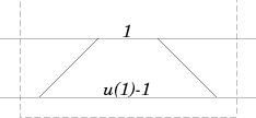
By substituting the second structure for the first, a bilinear form is obtained. The resulting bilinear form for a prime length DFT is

(4.8)

where , x=(x(0),⋯,x(p–1))^t, and where U_p is the matrix with the form

(4.9)

and V_p is the matrix with the form

(4.10)