13.1 F Distribution and One-Way ANOVA1
13.1.1 Student Learning Outcomes
By the end of this chapter, the student should be able to:
• Interpret the F probability distribution as the number of groups and the sample size change.
• Discuss two uses for the F distribution: One-Way ANOVA and the test of two variances.
• Conduct and interpret One-Way ANOVA.
• Conduct and interpret hypothesis tests of two variances.
13.1.2 Introduction
Many statistical applications in psychology, social science, business administration, and the natural sciences
involve several groups. For example, an environmentalist is interested in knowing if the average amount of
pollution varies in several bodies of water. A sociologist is interested in knowing if the amount of income a
person earns varies according to his or her upbringing. A consumer looking for a new car might compare
the average gas mileage of several models.
For hypothesis tests involving more than two averages, statisticians have developed a method called Anal-
ysis of Variance" (abbreviated ANOVA). In this chapter, you will study the simplest form of ANOVA called
single factor or One-Way ANOVA. You will also study the F distribution, used for One-Way ANOVA, and
the test of two variances. This is just a very brief overview of One-Way ANOVA. You will study this topic
in much greater detail in future statistics courses.
• One-Way ANOVA, as it is presented here, relies heavily on a calculator or computer.
• For further information about One-Way ANOVA, use the online link ANOVA2 . Use the back button
to return here. (The url is http://en.wikipedia.org/wiki/Analysis_of_variance.)
1This content is available online at <http://cnx.org/content/m17065/1.11/>.
2http://en.wikipedia.org/wiki/Analysis_of_variance
Available for free at Connexions <http://cnx.org/content/col10522/1.40>
583
584
CHAPTER 13. F DISTRIBUTION AND ONE-WAY ANOVA
13.2 One-Way ANOVA3
13.2.1 F Distribution and One-Way ANOVA: Purpose and Basic Assumptions of One-
Way ANOVA
The purpose of a One-Way ANOVA test is to determine the existence of a statistically significant difference
among several group means. The test actually uses variances to help determine if the means are equal or
not.
In order to perform a One-Way ANOVA test, there are five basic assumptions to be fulfilled:
• Each population from which a sample is taken is assumed to be normal.
• Each sample is randomly selected and independent.
• The populations are assumed to have equal standard deviations (or variances).
• The factor is the categorical variable.
• The response is the numerical variable.
13.2.2 The Null and Alternate Hypotheses
The null hypothesis is simply that all the group population means are the same. The alternate hypothesis
is that at least one pair of means is different. For example, if there are k groups:
Ho : µ 1 = µ 2 = µ 3 = ... = µ k
Ha : At least two of the group means µ 1, µ 2, µ 3, ..., µ k are not equal.
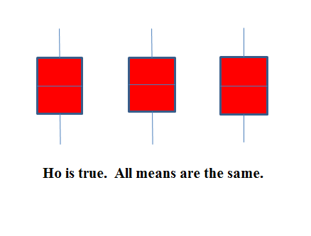
The graphs help in the understanding of the hypothesis test.
In the first graph (red box plots),
Ho : µ 1 = µ 2 = µ 3 and the three populations have the same distribution if the null hypothesis is true. The
variance of the combined data is approximately the same as the variance of each of the populations.
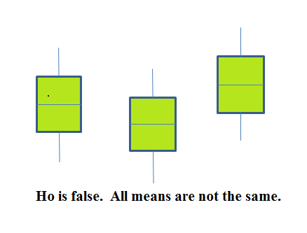
If the null hypothesis is false, then the variance of the combined data is larger which is caused by
the different means as shown in the second graph (green box plots).
3This content is available online at <http://cnx.org/content/m17068/1.10/>.
Available for free at Connexions <http://cnx.org/content/col10522/1.40>
585
13.3 The F Distribution and the F Ratio4
The distribution used for the hypothesis test is a new one. It is called the F distribution, named after Sir
Ronald Fisher, an English statistician. The F statistic is a ratio (a fraction). There are two sets of degrees of
freedom; one for the numerator and one for the denominator.
4This content is available online at <http://cnx.org/content/m17076/1.14/>.
Available for free at Connexions <http://cnx.org/content/col10522/1.40>
586
CHAPTER 13. F DISTRIBUTION AND ONE-WAY ANOVA
For example, if F follows an F distribution and the degrees of freedom for the numerator are 4 and the
degrees of freedom for the denominator are 10, then F ∼ F4,10.
NOTE: The F distribution is derived from the Student’s-t distribution. One-Way ANOVA expands
the t-test for comparing more than two groups. The scope of that derivation is beyond the level of
this course.
To calculate the F ratio, two estimates of the variance are made.
1. Variance between samples: An estimate of 2
σ that is the variance of the sample means multiplied by
n (when there is equal n). If the samples are different sizes, the variance between samples is weighted
to account for the different sample sizes. The variance is also called variation due to treatment or
explained variation.
2. Variance within samples: An estimate of 2
σ that is the average of the sample variances (also known
as a pooled variance). When the sample sizes are different, the variance within samples is weighted.
The variance is also called the variation due to error or unexplained variation.
• SSbetween = the sum of squares that represents the variation among the different samples.
• SSwithin = the sum of squares that represents the variation within samples that is due to chance.
To find a "sum of squares" means to add together squared quantities which, in some cases, may be weighted.
We used sum of squares to calculate the sample variance and the sample standard deviation in Descriptive
Statistics.
MS means "mean square." MSbetween is the variance between groups and MSwithin is the variance within
groups.
Calculation of Sum of Squares and Mean Square
• k = the number of different groups
• nj = the size of the jth group
• sj= the sum of the values in the jth group
• n = total number of all the values combined. (total sample size: ∑ nj)
• x = one value: ∑ x = ∑ sj
• Sum of squares of all values from every group combined: ∑ x2
• Between group variability: SStotal = ∑ x2 − (∑ x)2
n
• Total sum of squares: ∑ x2 − (∑ x)2
n
• Explained variation- sum of squares representing variation among the different samples SSbetween =
∑ (sj)2
(∑ s
−
j )2
nj
n
• Unexplained variation- sum of squares representing variation within samples due to chance:
SSwithin = SStotal − SSbetween
• df’s for different groups (df’s for the numerator): dfbetween = k − 1
• Equation for errors within samples (df’s for the denominator): dfwithin = n − k
• Mean square (variance estimate) explained by the different groups: MSbetween = SSbetween
dfbetween
• Mean square (variance estimate) that is due to chance (unexplained): MSwithin = SSwithin
dfwithin
MSbetween and MSwithin can be written as follows:
• MSbetween = SSbetween = SSbetween
d f between
k−1
• MSwithin = SSwithin = SSwithin
d f within
n−k
Available for free at Connexions <http://cnx.org/content/col10522/1.40>
587
The One-Way ANOVA test depends on the fact that MSbetween can be influenced by population differences
among means of the several groups. Since MSwithin compares values of each group to its own group mean,
the fact that group means might be different does not affect MSwithin.
The null hypothesis says that all groups are samples from populations having the same normal distribution.
The alternate hypothesis says that at least two of the sample groups come from populations with different
normal distributions. If the null hypothesis is true, MSbetween and MSwithin should both estimate the same
value.
NOTE: The null hypothesis says that all the group population means are equal. The hypothesis of
equal means implies that the populations have the same normal distribution because it is assumed
that the populations are normal and that they have equal variances.
F-Ratio or F Statistic
MS
F =
between
(13.1)
MSwithin
If MSbetween and MSwithin estimate the same value (following the belief that Ho is true), then the F-ratio
should be approximately equal to 1. Mostly just sampling errors would contribute to variations away
from 1. As it turns out, MSbetween consists of the population variance plus a variance produced from the
differences between the samples. MSwithin is an estimate of the population variance. Since variances are
always positive, if the null hypothesis is false, MSbetween will generally be larger than MSwithin. Then the
F-ratio will be larger than 1. However, if the population effect size is small it is not unlikely that MSwithin
will be larger in a give sample.
The above calculations were done with groups of different sizes. If the groups are the same size, the calcu-
lations simplify somewhat and the F ratio can be written as:
F-Ratio Formula when the groups are the same size
n · s_ 2
F =
x
(13.2)
s2pooled
where ...
• n =the sample size
• dfnumerator = k − 1
• dfdenominator = n − k
• s2pooled = the mean of the sample variances (pooled variance)
• s 2
x
= the variance of the sample means
The data is typically put into a table for easy viewing. One-Way ANOVA results are often displayed in this
manner by computer software.
Source of
Sum of Squares
Degrees of
Mean Square
F
Variation
(SS)
Freedom (df)
(MS)
continued on next page
Available for free at Connexions <http://cnx.org/content/col10522/1.40>
588
CHAPTER 13. F DISTRIBUTION AND ONE-WAY ANOVA
Factor
SS(Factor)
k - 1
MS(Factor) =
F =
(Between)
SS(Factor)/(k-1)
MS(Factor)/MS(Error)
Error
SS(Error)
n - k
MS(Error) =
(Within)
SS(Error)/(n-k)
Total
SS(Total)
n - 1
Table 13.1
Example 13.1
Three different diet plans are to be tested for mean weight loss. The entries in the table are the
weight losses for the different plans. The One-Way ANOVA table is shown below.
Plan 1
Plan 2
Plan 3
5
3.5
8
4.5
7
4
4
3.5
3
4.5
Table 13.2
One-Way ANOVA Table: The formulas for SS(Total), SS(Factor) = SS(Between) and SS(Error) =
SS(Within) are shown above. This same information is provided by the TI calculator hypothesis
test function ANOVA in STAT TESTS (syntax is ANOVA(L1, L2, L3) where L1, L2, L3 have the
data from Plan 1, Plan 2, Plan 3 respectively).
Source of
Sum of Squares
Degrees of
Mean Square
F
Variation
(SS)
Freedom (df)
(MS)
Factor
SS(Factor)
k - 1
MS(Factor)
F =
(Between)
= SS(Between)
= 3 groups - 1
= SS(Factor)/(k-1)
MS(Factor)/MS(Error)
=2.2458
= 2
= 2.2458/2
= 1.1229/2.9792
= 1.1229
= 0.3769
Error
SS(Error)
n - k
MS(Error)
(Within)
= SS(Within)
= 10 total data - 3
= SS(Error)/(n-k)
= 20.8542
groups
= 20.8542/7
= 7
= 2.9792
Total
SS(Total)
n - 1
= 2.9792 + 20.8542
= 10 total data - 1
=23.1
= 9
Table 13.3
The One-Way ANOVA hypothesis test is always right-tailed because larger F-values are way out in the
right tail of the F-distribution curve and tend to make us reject Ho.
Available for free at Connexions <http://cnx.org/content/col10522/1.40>
589
13.3.1 Notation
The notation for the F distribution is F ∼ Fdf(num),df(denom)
where df(num) = d f between and df(denom) = d f within
The mean for the F distribution is µ =
d f (num)
d f (denom)−1
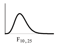
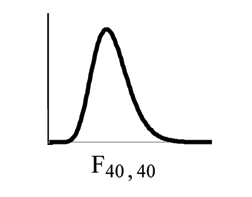
13.4 Facts About the F Distribution5
1. The curve is not symmetrical but skewed to the right.
2. There is a different curve for each set of dfs.
3. The F statistic is greater than or equal to zero.
4. As the degrees of freedom for the numerator and for the denominator get larger, the curve approxi-
mates the normal.
5. Other uses for the F distribution include comparing two variances and Two-Way Analysis of Variance.
Comparing two variances is discussed at the end of the chapter. Two-Way Analysis is mentioned for
your information only.
(a)
(b)
Figure 13.1
Example 13.2
One-Way ANOVA: Four sororities took a random sample of sisters regarding their grade means
for the past term. The results are shown below:
5This content is available online at <http://cnx.org/content/m17062/1.14/>.
Available for free at Connexions <http://cnx.org/content/col10522/1.40>
590
CHAPTER 13. F DISTRIBUTION AND ONE-WAY ANOVA
MEAN GRADES FOR FOUR SORORITIES
Sorority 1
Sorority 2
Sorority 3
Sorority 4
2.17
2.63
2.63
3.79
1.85
1.77
3.78
3.45
2.83
3.25
4.00
3.08
1.69
1.86
2.55
2.26
3.33
2.21
2.45
3.18
Table 13.4
Problem
Using a significance level of 1%, is there a difference in mean grades among the sororities?
Solution
Let µ 1, µ 2, µ 3, µ 4 be the population means of the sororities. Remember that the null hypothesis
claims that the sorority groups are from the same normal distribution. The alternate hypothesis
says that at least two of the sorority groups come from populations with different normal distri-
butions. Notice that the four sample sizes are each size 5.
NOTE: This is an example of a balanced design, since each factor (i.e. Sorority) has the same
number of observations.
Ho : µ 1 = µ 2 = µ 3 = µ 4
Ha: Not all of the means µ 1, µ 2, µ 3, µ 4 are equal.
Distribution for the test: F3,16
where k = 4 groups and n = 20 samples in total
d f (num) = k − 1 = 4 − 1 = 3
d f (denom) = n − k = 20 − 4 = 16
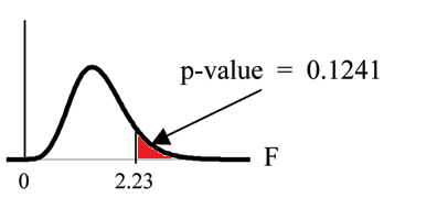
Calculate the test statistic: F = 2.23
Graph:
Available for free at Connexions <http://cnx.org/content/col10522/1.40>
591
Figure 13.2
Probability statement: p-value = P (F > 2.23) = 0.1241
Compare α and the p − value: α = 0.01
p-value = 0.1241
α < p-value
Make a decision: Since α < p-value, you cannot reject Ho.
Conclusion: There is not sufficient evidence to conclude that there is a difference among the mean
grades for the sororities.
TI-83+ or TI 84: Put the data into lists L1, L2, L3, and L4. Press ❙❚❆❚ and arrow over to ❚❊❙❚❙.
Arrow down to ❋✿❆◆❖❱❆. Press ❊◆❚❊❘ and Enter (▲✶✱▲✷✱▲✸✱▲✹). The F statistic is 2.2303 and the
p-value is 0.1241. df(numerator) = 3 (under ✧❋❛❝t♦r✧) and df(denominator) = 16 (under ❊rr♦r).
Example 13.3
A fourth grade class is studying the environment. One of the assignments is to grow bean plants
in different soils. Tommy chose to grow his bean plants in soil found outside his classroom mixed
with dryer lint. Tara chose to grow her bean plants in potting soil bought at the local nursery.
Nick chose to grow his bean plants in soil from his mother’s garden. No chemicals were used
on the plants, only water. They were grown inside the classroom next to a large window. Each
child grew 5 plants. At the end of the growing period, each plant was measured, producing the
following data (in inches):
Tommy’s Plants
Tara’s Plants
Nick’s Plants
24
25
23
21
31
27
23
23
22
30
20
30
23
28
20
Table 13.5
Available for free at Connexions <http://cnx.org/content/col10522/1.40>
592
CHAPTER 13. F DISTRIBUTION AND ONE-WAY ANOVA
Problem 1
Does it appear that the three media in which the bean plants were grown produce the same mean
height? Test at a 3% level of significance.
Solution
This time, we will perform the calculations that lead to the F’ statistic. Notice that each group has
2
the same number of plants so we will use the formula F’ = n·s_x .
s2pooled
First, calculate the sample mean and sample variance of each group.
Tommy’s Plants
Tara’s Plants
Nick’s Plants
Sample Mean
24.2
25.4
24.4
Sample Variance
11.7
18.3
16.3
Table 13.6
Next, calculate the variance of the three group means (Calculate the variance of 24.2, 25.4, and
24.4). Variance of the group means = 0.413 = s 2
x
Then MS
2
between = nsx
= (5) (0.413) where n = 5 is the sample size (number of plants each child
grew).
Calculate the mean of the three sample variances (Calculate the mean of 11.7, 18.3, and 16.3). Mean
of the sample variances = 15.433 = s2pooled
Then MSwithin = s2pooled = 15.433.
2
The F statistic (or F ratio) is F = MSbetween = n·s_x
= (5)·(0.413) = 0.134
MSwithin
s2
15.433
pooled
The dfs for the numerator = the number of groups − 1 = 3 − 1 = 2
The dfs for the denominator = the total number of samples − the number of groups = 15 − 3 = 12
The distribution for the test is F2,12 and the F statistic is F = 0.134
The p-value is P (F > 0.134) = 0.8759.
Decision: Since α = 0.03 and the p-value = 0.8759, do not reject Ho. (Why?)
Conclusion: With a 3% the level of significance, from the sample data, the evidence is not sufficient
to conclude that the mean heights of the bean plants are different.
(This experiment was actually done by three classmates of the son of one of the authors.)
Another fourth grader also grew bean plants but this time in a jelly-like mass. The heights were
(in inches) 24, 28, 25, 30, and 32.
Problem 2
(Solution on p. 610.)
Do a One-Way ANOVA test on the 4 groups. You may use your calculator or computer to
perform the test. Are the heights of the bean plants different? Use a solution sheet (Section 14.5.4).
Available for free at Connexions <http://cnx.org/content/col10522/1.40>
593
13.4.1 Optional Classroom Activity
From the class, create four groups of the same size as follows: men under 22, men at least 22, women under
22, women at least 22. Have each member of each group record the number of states in the United States
he or she has visited. Run an ANOVA test to determine if the average number of states visited in the four
groups are the same. Test at a 1% level of significance. Use one of the solution sheets (Section 14.5.4) at the
end of the chapter (after the homework).
13.5 Test of Two Variances6
Another of the uses of the F distribution is testing two variances. It is often desirable to compare two
variances rather than two averages. For instance, college administrators would like two college professors
grading exams to have the same variation in their grading. In order for a lid to fit a container, the variation
in the lid and the container should be the same. A supermarket might be interested in the variability of
check-out times for two checkers.
In order to perform a F test of two variances, it is important that the following are true:
1. The populations from which the two samples are drawn are normally distributed.
2. The two populations are independent of each other.
Suppose we sample randomly from two independent normal populations. Let 2
2