We can divide mathematics into pure and applied maths. Pure maths is the theory of maths and is very abstract. The work you have covered on algebra is mostly pure maths. Applied maths is all about taking the theory (or pure maths) and applying it to the real world. To be able to do applied maths, you first have to learn pure maths.
But what does this have to do with probability? Well, just as mathematics can be divided into pure maths and applied maths, so statistics can be divided into probability theory and applied statistics. And just as you cannot do applied mathematics without knowing any theory, you cannot do statistics without beginning with some understanding of probability theory. Furthermore, just as it is not possible to describe what arithmetic is without describing what mathematics as a whole is, it is not possible to describe what probability theory is without some understanding of what statistics as a whole is about, and statistics, in its broadest sense, is about 'processes'.
Galileo wrote down some ideas about dice games in the seventeenth century. Since then many discussions and papers have been written about probability theory, but it still remains a poorly understood part of mathematics.
A process is how an object changes over time. For example, consider a coin. Now, the coin by itself is not a process; it is simply an object. However, if I was to flip the coin (i.e. putting it through a process), after a certain amount of time (however long it would take to land), it is brought to a final state. We usually refer to this final state as 'heads' or 'tails' based on which side of the coin landed face up, and it is the 'heads' or 'tails' that the statistician (person who studies statistics) is interested in. Without the process there is nothing to examine. Of course, leaving the coin stationary is also a process, but we already know that its final state is going to be the same as its original state, so it is not a particularly interesting process. Usually when we speak of a process, we mean one where the outcome is not yet known, otherwise there is no real point in analyzing it. With this understanding, it is very easy to understand what, precisely, probability theory is.
When we speak of probability theory as a whole, we mean the way in which we quantify the possible outcomes of processes. Then, just as 'applied' mathematics takes the methods of 'pure' mathematics and applies them to real-world situations, applied statistics takes the means and methods of probability theory (i.e. the means and methods used to quantify possible outcomes of events) and applies them to real-world events in some way or another. For example, we might use probability theory to quantify the possible outcomes of the coin-flip above as having a 50% chance of coming up heads and a 50% chance of coming up tails, and then use statistics to apply it a real-world situation by saying that of six coins sitting on a table, the most likely scenario is that three coins will come up heads and three coins will come up tails. This, of course, may not happen, but if we were only able to bet on ONE outcome, we would probably bet on that because it is the most probable. But here, we are already getting ahead of ourselves. So let's back up a little.
To quantify results, we may use a variety of methods, terms, and notations, but a few common ones are:
a percentage (for example '50%')
a proportion of the total number of outcomes (for example, '5/10')
a proportion of 1 (for example, '1/2')
You may notice that all three of the above examples represent the same probability, and in fact ANY method of probability is fundamentally based on the following procedure:
Define a process.
Define the total measure for all outcomes of the process.
Describe the likelihood of each possible outcome of the process with respect to the total measure.
The term 'measure' may be confusing, but one may think of it as a ruler. If we take a ruler that is 1 metre long, then half of that ruler is 50 centimetres, a quarter of that ruler is 25 centimetres, etc. However, the thing to remember is that without the ruler, it makes no sense to talk about proportions of a ruler! Indeed, the three examples above (50%, 5/10, and 1/2) represented the same probability, the only difference was how the total measure (ruler) was defined. If we go back to thinking about it in terms of a ruler '50%' means '50/100', so it means we are using 50 parts of the original 100 parts (centimetres) to quantify the outcome in question. '5/10' means 5 parts out of the original 10 parts (10 centimetre pieces) depict the outcome in question. And in the last example, '1/2' means we are dividing the ruler into two pieces and saying that one of those two pieces represents the outcome in question. But these are all simply different ways to talk about the same 50 centimetres of the original 100 centimetres! In terms of probability theory, we are only interested in proportions of a whole.
Although there are many ways to define a 'measure', the most common and easiest one to generalize is to use '1' as the total measure. So if we consider the coin-flip, we would say that (assuming the coin was fair) the likelihood of heads is 1/2 (i.e. half of one) and the likelihood of tails is 1/2. On the other hand, if we consider the event of not flipping the coin, then (assuming the coin was originally heads-side-up) the likelihood of heads is now 1, while the likelihood of tails is 0. But we could have also used '14' as the original measure and said that the likelihood of heads or tails on the coin-flip was each '7 out of 14', while on the non-coin-flip the likelihood of heads was '14 out of 14', and the likelihood of tails was '0 out of 14'. Similarly, if we consider the throwing of a (fair) six-sided die, it may be easiest to set the total measure to '6' and say that the likelihood of throwing a '4' is '1 out of the 6', but usually we simply say that it is 1/6, i.e. '1/6 of 1'.
There are three important concepts associated with a random experiment: 'outcome', 'sample space', and 'event'. Two examples of experiments will be used to familiarize you with these terms:
In Experiment 1 a single die is thrown and the value of the top face after it has come to rest is noted.
In Experiment 2 two dice are thrown at the same time and the total of the values of each of the top faces after they have come to rest is noted.
An outcome of an experiment is a single result of that experiment.
A possible outcome of Experiment 1: the value on the top face is '3'
A possible outcome of Experiment 2: the total value on the top faces is '9'
The sample space of an experiment is the complete set of possible outcomes of the experiment.
Experiment 1: the sample space is 1,2,3,4,5,6
Experiment 2: the sample space is 2,3,4,5,6,7,8,9,10,11,12
If you roll two die and add the results, the most common outcome is 7. To understand this, think that there is only one way to get 2 as a result (both dice landing with 1) and there is only way to get 12 as a result (both dice landing with 6). The opposite sides of a six sided dice add up to 7. From this you should be able to work out that there are 12 ways to get a 7.
An event is any set of outcomes of an experiment.
A possible event of Experiment 1: an even number being on the top face of the die
A possible event of Experiment 2: the numbers on the top face of each die being equal
The term random experiment or statistical experiment is used to describe any repeatable process, the results of which are analyzed in some way. For example, flipping a coin and noting whether or not it lands heads-up is a random experiment because the process is repeatable. On the other hand, your reading this sentence for the first time and noting whether you understand it is not a random experiment because it is not repeatable (though making a number of random people read it and noting which ones understand it would turn it into a random experiment).
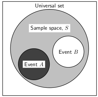
A Venn diagram can be used to show the relationship between the possible outcomes of a random experiment and the sample space. The Venn diagram in Figure 12.1 shows the difference between the universal set, a sample space and events and outcomes as subsets of the sample space.
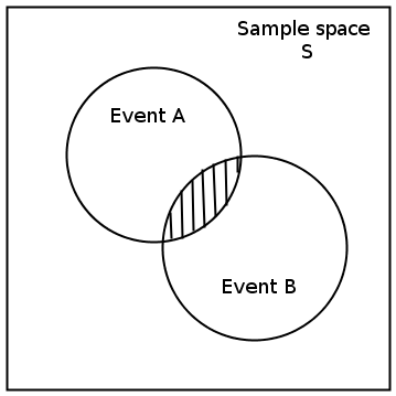
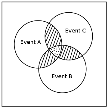
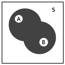
We can draw Venn diagrams for experiments with two and three events. These are shown in Figure 12.2 and Figure 12.3. Venn diagrams for experiments with more than three events are more complex and are not covered at this level.
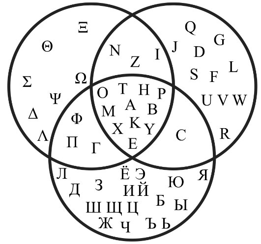
The Greek, Russian and Latin alphabets can be illustrated using Venn diagrams. All these alphabets have some common letters. The Venn diagram is given below:
The union of
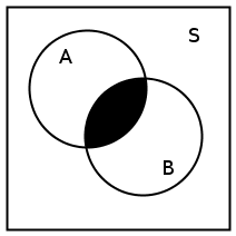
A and B is the set of all elements in A or in B (or in both).  is also written A∪B. The intersection of A and B is the set of all elements in both
A and B.
is also written A∪B. The intersection of A and B is the set of all elements in both
A and B.
 is also written as A∩B.
Venn diagrams can also be used to indicate the union and intersection between events in a sample space (Figure 12.5 and Figure 12.6).
We use n(S) to refer to the number of elements in a set S, n(X) for the number of elements in X, etc.
In a box there are pieces of paper with the numbers from 1 to 9 written on them. A piece of paper is drawn from the box and the number on it is noted. Let S denote the sample space, let P denote the event 'drawing a prime number', and let E denote the event 'drawing an even number'. Using appropriate notation, in how many ways is it possible to draw: i) any number? ii) a prime number? iii) an even number? iv) a number that is either prime or even? v) a number that is both prime and even?
Consider the events: :
Drawing a prime number: P={2;3;5;7 }
Drawing an even number: E={2;4;6;8 }
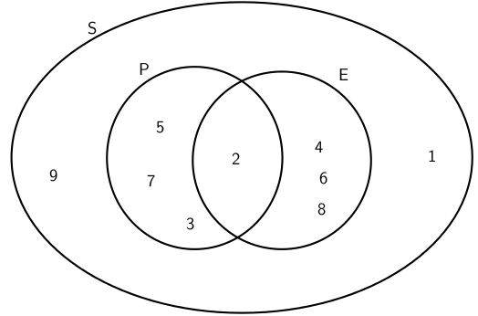
The union of P and E is the set of all elements in P or in E (or in both). P∪E=2,3,4,5,6,7,8 .
The intersection of P and E is the set of all elements in both P and E. P∩E=2.
Find the number in each set :

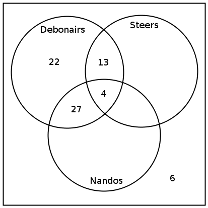
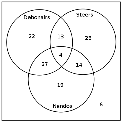
100 people were surveyed to find out which fast food chain (Nandos, Debonairs or Steers) they preferred. The following results were obtained:
50 liked Nandos
66 liked Debonairs
40 liked Steers
27 liked Nandos and Debonairs but not Steers
13 liked Debonairs and Steers but not Nandos
4 liked all three
94 liked at least one
How many people did not like any of the fast food chains?
How many people liked Nandos and Steers, but not Debonairs?
Draw a Venn diagram: The number of people who liked Nandos and Debonairs is 27, so this is the intersection of these two events. The number of people who liked Debonairs and Steers is 13, so the intersection of Debonairs and Steers is 13. We are told that 4 people like all three options, and so this means that there are 4 people in the intersection of all three options. So we can work out that the number of people who like just Debonairs is 66–4–27–13=22 (This is simply the total number who like Debonairs minus the number of people who like Debonairs and Steers, or Debonairs and Nandos or all three). We draw the following diagram to represent the data:
Work out how many people like none: We are told that there were 100 people and that 94 liked at least one. So the number of people that liked none is: 100–94=6. This is the answer to a).
Work out how many like Nandos and Steers but not Debonairs: We can redraw the part of the Venn diagram that is of interest:
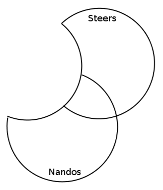
Total people who like Nandos: 50
Of these 27 like both Nandos and Debonairs, and 4 people like all three options. So we find that the total number of people who just like Nandos is: 50–27–4=19
Total people who like Steers: 40
Of these 13 like both Steers and Debonairs, and 4 like all three options. So we find that the total number of people who like just Steers is: 40–13–4=23
Now use the identity n(N or S)=n(N)+n(S)–n(N and S) to find the number of people who like Nandos and Steers, but not Debonairs.

The Venn diagram with that represents all this information is given:
Which cellphone networks have you used or are you signed up for (e.g. Vodacom, Mtn or CellC)? Collect this information from your classmates as well. Then use the information to draw a Venn diagram (if you have more than three networks, then choose only the three most popular or draw Venn diagrams for all the combinations). Try to see if you can work out the number of people who use just one network, or the number of people who use all the networks.
A final notion that is important to understand is the notion
of complement.
Just as in geometry when two angles are called 'complementary' if they added up
to 90 degrees, (the two angles 'complement' each other to make a right angle), the complement of a set of outcomes A is the set of all outcomes in the sample space but not in A. It is usually denoted
A' (or sometimes AC), and called 'the complement of A' or simply 'A-complement'. Because it refers to the set of everything outside of A, it is also often referred to as 'not-A'. Thus, by definition, if S denotes the entire sample space of possible outcomes, and A is any subset of outcomes that we are interested in (i.e. an event), then A∪A' = S is always
true, (i.e. A' complements A to form the entire
sample space). So in the exercise above,  ,
while
,
while  . So
. So 
The probability of a complementary event refers to the probability associated with the complement of an event, i.e. the probability that something other than the event in question will occur. For example, if P(A)=0,25, then the probability of A not occurring is the probability associated with all other events in <