As we will see later in this course, there now exist a wide variety of approaches to recover a sparse signal x from a small number of linear measurements. We begin by considering a natural first approach to the problem of sparse recovery.

Given measurements y=Φx and the knowledge that our original signal x is sparse or compressible, it is natural to attempt to recover x by solving an optimization problem of the form

(4.1)

where B(y) ensures that is consistent with the measurements y. Recall that ∥z∥₀=| supp (z)| simply counts the number of nonzero entries in z, so Equation 4.1 simply seeks out the sparsest signal consistent with the observed measurements. For example, if our measurements are exact and noise-free, then we can set B(y)={z:Φz=y}. When the measurements have been contaminated with a small amount of bounded noise, we could instead set . In both cases, Equation 4.1 finds the sparsest x that is consistent with the measurements y.

Note that in Equation 4.1 we are inherently assuming that x itself is sparse. In the more common setting where x=Ψα, we can easily modify the approach and instead consider

(4.2)

where B(y)={z:ΦΨz=y} or . By setting we see that Equation 4.1 and Equation 4.2 are essentially identical. Moreover, as noted in "Matrices that satisfy the RIP", in many cases the introduction of Ψ does not significantly complicate the construction of matrices Φ such that will satisfy the desired properties. Thus, for most of the remainder of this course we will restrict our attention to the case where Ψ=I. It is important to note, however, that this restriction does impose certain limits in our analysis when Ψ is a general dictionary and not an orthonormal basis. For example, in this case , and thus a bound on cannot directly be translated into a bound on , which is often the metric of interest.

Although it is possible to analyze the performance of Equation 4.1 under the appropriate assumptions on Φ, we do not pursue this strategy since the objective function ∥·∥₀ is nonconvex, and hence Equation 4.1 is potentially very difficult to solve. In fact, one can show that for a general matrix Φ, even finding a solution that approximates the true minimum is NP-hard. One avenue for translating this problem into something more tractable is to replace ∥·∥₀ with its convex approximation ∥·∥₁. Specifically, we consider

(4.3)

Provided that B(y) is convex, Equation 4.3 is computationally feasible. In fact, when B(y)={z:Φz=y}, the resulting problem can be posed as a linear program 2.

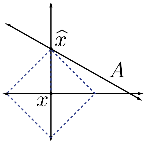(a) Approximation in ℓ1 norm

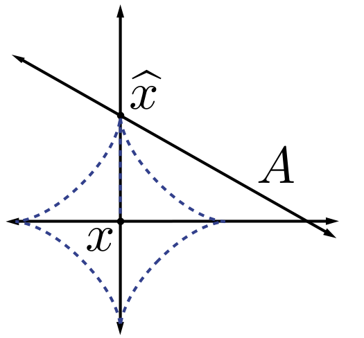(b) Approximation in ℓp quasinorm

Figure 4.1. 

Best approximation of a point in R² by a a one-dimensional subspace using the ℓ₁ norm and the ℓ_p quasinorm with .

It is clear that replacing Equation 4.1 with Equation 4.3 transforms a computationally intractable problem into a tractable one, but it may not be immediately obvious that the solution to Equation 4.3 will be at all similar to the solution to Equation 4.1. However, there are certainly intuitive reasons to expect that the use of ℓ₁ minimization will indeed promote sparsity. As an example, recall the example we discussed earlier shown in Figure 4.1. In this case the solutions to the ℓ₁ minimization problem coincided exactly with the solution to the ℓ_p minimization problem for any p<1, and notably, is sparse. Moreover, the use of ℓ₁ minimization to promote or exploit sparsity has a long history, dating back at least to the work of Beurling on Fourier transform extrapolation from partial observations 1.

Additionally, in a somewhat different context, in 1965 Logan 4 showed that a bandlimited signal can be perfectly recovered in the presence of arbitrary corruptions on a small interval. Again, the recovery method consists of searching for the bandlimited signal that is closest to the observed signal in the ℓ₁ norm. This can be viewed as further validation of the intuition gained from Figure 4.1 — the ℓ₁ norm is well-suited to sparse errors.

Historically, the use of ℓ₁ minimization on large problems finally became practical with the explosion of computing power in the late 1970's and early 1980's. In one of its first applications, it was demonstrated that geophysical signals consisting of spike trains could be recovered from only the high-frequency components of these signals by exploiting ℓ₁ minimization 3, 6, 8. Finally, in the 1990's there was renewed interest in these approaches within the signal processing community for the purpose of finding sparse approximations to signals and images when represented in overcomplete dictionaries or unions of bases 2, 5. Separately, ℓ₁ minimization received significant attention in the statistics literature as a method for variable selection in linear regression, known as the Lasso 7.

Thus, there are a variety of reasons to suspect that ℓ₁ minimization will provide an accurate method for sparse signal recovery. More importantly, this also provides a computationally tractable approach to the sparse signal recovery problem. We now provide an overview of ℓ₁ minimization in both the noise-free and noisy settings from a theoretical perspective. We will then further discuss algorithms for performing ℓ₁ minimization later in this course.

We now begin our analysis of

(4.4)

for various specific choices of B(y). In order to do so, we require the following general result which builds on Lemma 4 from "ℓ₁ minimization proof". The key ideas in this proof follow from 1.

Suppose that Φ satisfies the restricted isometry property (RIP) of order 2K with . Let be given, and define . Let Λ₀ denote the index set corresponding to the K entries of x with largest magnitude and Λ₁ the index set corresponding to the K entries of h_Λ0^c with largest magnitude. Set Λ=Λ₀∪Λ₁. If , then

(4.5)

where

(4.6)

Proof

We begin by observing that h=h_Λ+h_Λ^c, so that from the triangle inequality

(4.7) ∥h∥₂ ≤ ∥h_Λ∥₂ + ∥h_Λ^c∥₂ .

We first aim to bound ∥h_Λ^c∥₂. From Lemma 3 from "ℓ₁ minimization proof" we have

(4.8)

where the Λ_j are defined as before, i.e., Λ₁ is the index set corresponding to the K largest entries of h_Λ0^c (in absolute value), Λ₂ as the index set corresponding to the next K largest entries, and so on.

We now wish to bound ∥h_Λ0^c∥₁. Since , by applying the triangle inequality we obtain

(4.9)

Rearranging and again applying the triangle inequality,

(4.10)

Recalling that σ_K(x)₁=∥x_Λ0^c∥₁=∥x – x_Λ0∥₁,

(4.11) ∥h_Λ0^c∥₁ ≤ ∥h_Λ0∥₁ + 2 σ_K ( x ) ₁ .

Combining this with Equation 4.8 we obtain

(4.12)

where the last inequality follows from standard bounds on ℓ_p norms (Lemma 1 from "The RIP and the NSP"). By observing that ∥h_Λ0∥₂≤∥h_Λ∥₂ this combines with Equation 4.7 to yield

(4.13)

We now turn to establishing a bound for ∥h_Λ∥₂. Combining Lemma 4 from "ℓ₁ minimization proof" with Equation 4.11 and again applying standard bounds on ℓ_p norms we obtain

(4.14)

Since ∥h_Λ0∥₂≤∥h_Λ∥₂,

(4.15)

The assumption that ensures that α<1. Dividing by

Page 1Page 2Page 3Page 4Page 5Page 6Page 7Page 8Page 9Page 10Page 11Page 12Page 13

PREV   NEXT