2013/02/11 14:59:07 -0600
In many applications, one never has to deal directly with the scaling functions or wavelets. Only the coefficients h(n) and h1(n) in the defining equations Equation 3.13 and Equation 3.24 and c(k) and dj(k) in the expansions Equation 3.28, Equation 3.29, and Equation 3.30 need be considered, and they can be viewed as digital filters and digital signals respectively 7, 26. While it is possible to develop most of the results of wavelet theory using only filter banks, we feel that both the signal expansion point of view and the filter bank point of view are necessary for a real understanding of this new tool.
In order to work directly with the wavelet transform coefficients, we will derive the relationship between the expansion coefficients at a lower scale level in terms of those at a higher scale. Starting with the basic recursion equation from Equation 3.13

and assuming a unique solution exists, we scale and translate the time variable to give

which, after changing variables m=2k+n, becomes

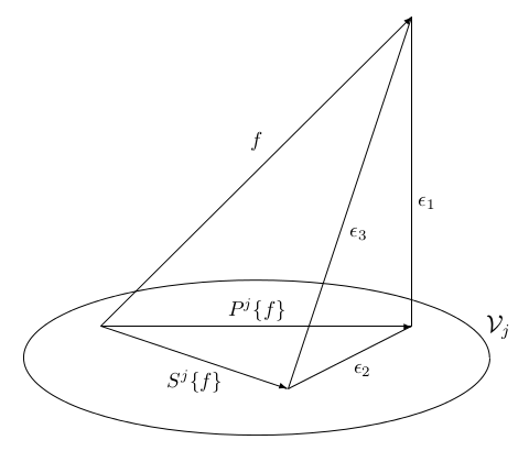
If we denote Vj as

then

is expressible at a scale of j+1 with scaling functions only and no wavelets. At one scale lower resolution, wavelets are necessary for the “detail" not available at a scale of j. We have

where the 2j/2 terms maintain the unity norm of the basis functions at various scales. If φj,k(t) and ψj,k(t) are orthonormal or a tight frame, the j level scaling coefficients are found by taking the inner product

which, by using Equation 4.3 and interchanging the sum and integral, can be written as

but the integral is the inner product with the scaling function at a scale of j+1 giving

The corresponding relationship for the wavelet coefficients is

In the discipline of digital signal processing, the “filtering" of a sequence of numbers (the input signal) is achieved by convolving the sequence with another set of numbers called the filter coefficients, taps, weights, or impulse response. This makes intuitive sense if you think of a moving average with the coefficients being the weights. For an input sequence x(n) and filter coefficients h(n), the output sequence y(n) is given by

There is a large literature on digital filters and how to design them 19, 18. If the number of filter coefficients N is finite, the filter is called a Finite Impulse Response (FIR) filter. If the number is infinite, it is called an Infinite Impulse (IIR) filter. The design problem is the choice of the h(n) to obtain some desired effect, often to remove noise or separate signals 18, 19.
In multirate digital filters, there is an assumed relation between the integer index n in the signal x(n) and time. Often the sequence of numbers are simply evenly spaced samples of a function of time. Two basic operations in multirate filters are the down-sampler and the up-sampler. The down-sampler (sometimes simply called a sampler or a decimator) takes a signal x(n) as an input and produces an output of y(n)=x(2n). This is symbolically shown in Figure 4.1. In some cases, the down-sampling is by a factor other than two and in some cases, the output is the odd index terms y(n)=x(2n+1), but this will be explicitly stated if it is important.
In down-sampling, there is clearly the possibility of losing information since half of the data is discarded. The effect in the frequency domain (Fourier transform) is called aliasing which states that the result of this loss of information is a mixing up of frequency components 19, 18. Only if the original signal is band-limited (half of the Fourier coefficients are zero) is there no loss of information caused by down-sampling.
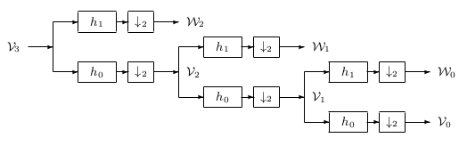
We talk about digital filtering and down-sampling because that is exactly what Equation 4.9 and Equation 4.10 do. These equations show that the scaling and wavelet coefficients at different levels of scale can be obtained by convolving the expansion coefficients at scale j by the time-reversed recursion coefficients h(–n) and h1(–n) then down-sampling or decimating (taking every other term, the even terms) to give the expansion coefficients at the next level of j–1. In other words, the scale-j coefficients are “filtered" by two FIR digital filters with coefficients h(–n) and h1(–n) after which down-sampling gives the next coarser scaling and wavelet coefficients. These structures implement Mallat's algorithm 16, 15 and have been developed in the engineering literature on filter banks, quadrature mirror filters (QMF), conjugate filters, and perfect reconstruction filter banks 20, 21, 27, 29, 28, 25, 26 and are expanded somewhat in Chapter: Filter Banks and Transmultiplexers of this book. Mallat, Daubechies, and others showed the relation of wavelet coefficient calculation and filter banks. The implementation of Equation 4.9 and Equation 4.10 is illustrated in Figure 4.2 where the down-pointing arrows denote a decimation or down-sampling by two and the other boxes denote FIR filtering or a convolution by h(–n) or h1(–n). To ease notation, we use both h(n) and h0(n) to denote the scaling function coefficients for the dilation equation Equation 3.13.
As we will see in Chapter: The Scaling Function and Scaling Coefficients, Wavelet and Wavelet Coefficients , the FIR filter implemented by h(–n) is a lowpass filter, and the one implemented by h1(–n) is a highpass filter. Note the average number of data points out of this system is the same as the number in. The number is doubled by having two filters; then it is halved by the decimation back to the original number. This means there is the possibility that no information has been lost and it will be possible to completely recover the original signal. As we shall see, that is indeed the case. The aliasing occurring in the upper bank can be “undone" or cancelled by using the signal from the lower bank. This is the idea behind perfect reconstruction in filter bank theory 26, 6.
This splitting, filtering, and decimation can be repeated on the scaling coefficients to give the two-scale structure in Figure 4.3. Repeating this on the scaling coefficients is called iterating the filter bank. Iterating the filter bank again gives us the three-scale structure in Figure 4.4.
The frequency response of a digital filter is the discrete-time Fourier transform of its impulse response (coefficients) h(n). That is given by

The magnitude of this complex-valued function gives the ratio of the output to the input of the filter for a sampled sinusoid at a frequency of ω in radians per seconds. The angle of H(ω) is the phase shift between the output and input.
The first stage of two banks divides the spectrum of cj+1(k) into a lowpass and highpass band, resulting in the scaling coefficients and wavelet coefficients at lower scale cj(k) and dj(k). The second stage then divides that lowpass band into another lower lowpass band and a bandpass band. The first stage divides the spectrum into two equal parts. The second stage divides the lower half into quarters and so on. This results in a logarithmic set of bandwidths as illustrated in Figure 4.5. These are called “constant-Q" filters in filter bank language because the ratio of the band width to the center frequency of the band is constant. It is also interesting to note that a musical scale defines octaves in a similar way and that the ear responds to frequencies in a similar logarithmic fashion.
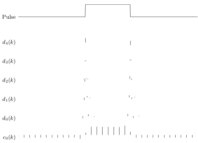
For any practical signal that is bandlimited, there will be an upper scale j=J, above which the wavelet coefficients, dj(k), are negligibly small 9. By starting with a high resolution description of a signal in terms of the scaling coefficients cJ, the analysis tree calculates the DWT
down to as low a resolution, j=j0, as desired by having J–j0 stages. So, for f(t)∈VJ, using Equation 3.8 we have

which is a finite scale version of Equation 3.33. We will discuss the choice of j0 and J further in Chapter: Calculation of the Discrete Wavelet Transform.
As one would expect, a reconstruction of the original fine scale coefficients of the signal can be made from a combination of the scaling function and wavelet coefficients at a coarse resolution. This is derived by considering a signal in the j+1 scaling function space f(t)∈Vj+1. This function can be written in terms of the scaling function as

or in terms of the next scale (which also requires wavelets) as

Substituting Equation 4.1 and m45094 into Equation 4.15 gives

Because all of these functions are orthonormal, multiplying Equation 4.14 and
Equation 4.16 by  and integrating evaluates the
coefficient as
and integrating evaluates the
coefficient as

For synthesis in the filter bank we have a sequence of first up-sampling or stretching, then filtering. This means that the input to the filter has zeros inserted between each of the original terms. In other words,

where the input signal is stretched to twice its original length and zeros are inserted. Clearly this up-sampling or stretching could be done with factors other than two, and the two equation above could have the x(n) and 0 reversed. It is also clear that up-sampling does not lose any information. If you first up-sample then down-sample, you are back where you started. However, if you first down-sample then up-sample, you are not generally back where you started.
Our reason for discussing filtering and up-sampling here is that
is exactly what the synthesis operation Equation 4.17 does.
This equation is evaluated by up-sampling the j scale coefficient
sequence cj(k), which means double its length by inserting zeros
between each term, then convolving it with the scaling coefficients
h(n). The same is done to the j level wavelet coefficient sequence
and the results are added to give the j+1 level scaling function
coefficients. This structure is illustrated in Figure 4.6 where
g0(n)=h(