227
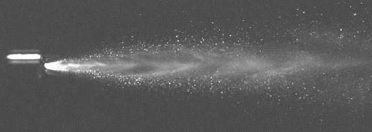
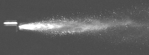
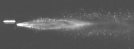
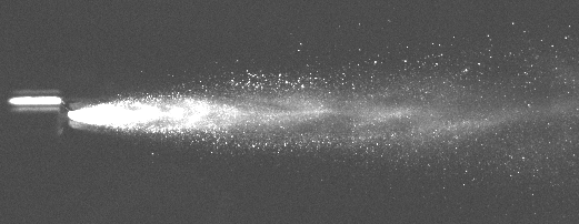
Fig. 4. Consecutive high speed images showing the pulsation effect from an injection nozzle.
A frequency of 1000 Hz was used in the imaging. The pulsation frequency was measured as 50 Hz.
Although high-speed cameras are sensitive equipment, they have sufficient portability
that we have used them in outside-the-lab environments at reasonable ambient
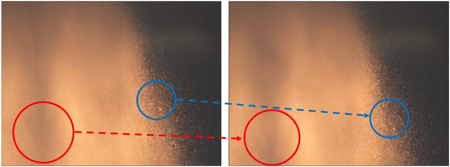
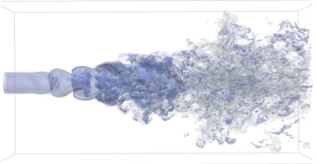
conditions. Figure 5, for instance, shows consecutive images of a dense air-assisted spray
that was running in the nozzle test stand. The velocity profile was needed for boundary
conditions of a CFD model. Velocities of 60 – 100 ft/s were measured, with the magnitude
dependent on the location. In dense sprays, reasonable estimates for velocity can be
provided by watching the motion of flow features in the spray, then applying velocimetric
principles [Raffel et al., 1998]. Near the edge, tracking the motion of groups of individual drops is also useful.

228
Applied Computational Fluid Dynamics
Fig. 5. High speed images (1000 Hz) showing how flow features and collections of drops are used to estimate velocity locally using velocimetry principles. This example is from a dense air-assisted spray located outside the authors’ laboratory, hence outside the realm of our
laser diagnostics.
2.3 PLIF imaging
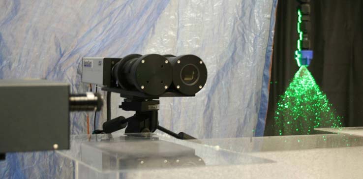
When a small amount of a fluorescent dye is added to the feed liquid, Planar Laser-Induced
Fluorescence (PLIF) can be used to capture detailed images of the spray as it issues from the nozzle. A plane of pulsed laser light (duration 10 ns) is aligned to pass through the axis of the spray. A camera is aligned perpendicular to the laser plane. The system is synchronized
so that the laser pulsates while the camera shutter is open. Figure 6 shows a photographic
Fig. 6. Photograph taken during a PLIF imaging experiment utilizing a Dantec Dynamics FlowMap System Hub.
Industrial Sprays: Experimental Characterization and Numerical Modeling
229
image taken during a PLIF experiment to best illustrate the method. In velocimetry mode,
dual images using dual laser pulses are taken on the order of 10 to 100 µs apart. The
movement of the spray structure or droplets themselves over the known time increment is
used to calculate the local velocity. The method has been shown to give consistent velocity
results before, during, and after the droplet formation. The velocity distribution can give
some information on expected mass flux pattern. However, the method doesn’t distinguish
between large and small droplets or account for the variable spatial concentration of
droplets, so strictly speaking an actual flux cannot be computed from the velocity vector
results. Averaging of many PLIF images can give useful information on mass flux within the
slice of the spray that is illuminated.
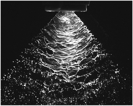
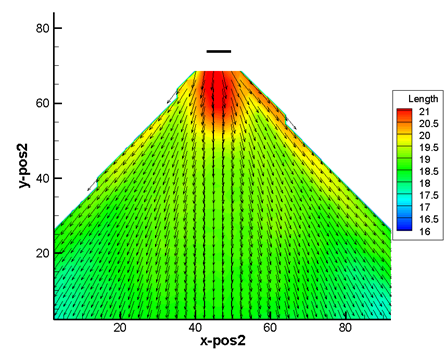
Figure 7 shows a PLIF image of an agricultural spray and the corresponding averaged
velocimetric data taken from 500 image pairs. The vectors form a fairly continuous contour
that is consistent with the characteristic shouldering of the spray flux.
Fig. 7. Left, example PLIF image of a flat fan agricultural spray, Spraying Systems Co. TeeJet 8002. Right, velocity contour plot with overlaid vectors, average of 500 image pairs.
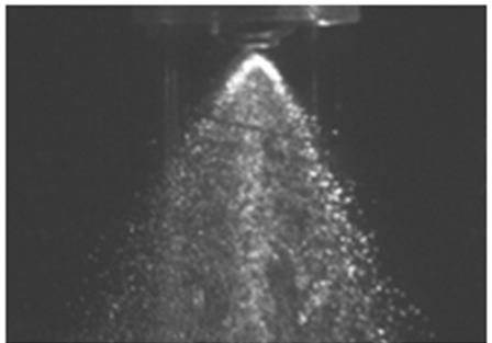
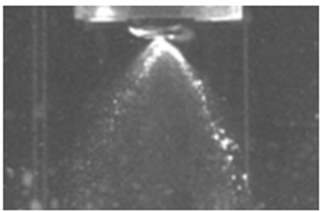
Figure 8 shows PLIF imaging of the same spray as is shown in the high-speed images of
Figure 4. The short 10 ns duration of the laser is sufficient to provide rich detail on the spray structure. The pulsating nature of the spray is again evident by comparing images. The PLIF
image allows quantitative calculations to estimate the amount of mass issued in the pulses
(or “surges”) compared to the baseline flow between pulses.
Figure 9 shows a comparison of Mie Scattering and PLIF imaging. The Mie Scattering is
sensitive to surface area whereas PLIF imaging is proportional to volume. It is easily noted that a large fraction of the spray volume is present on the outside edges of the spray, and at the same time there are many small droplets present in the interior portion.
230
Applied Computational Fluid Dynamics
Fig. 8. For the identical nozzle as shown in Figure 4, PLIF imaging at 5 Hz was used to better understand the flow characteristics during and between pulsations.
Industrial Sprays: Experimental Characterization and Numerical Modeling
231
Fig. 9. Mie Scattering (left) and PLIF (right) images, showing surface area versus volume
effect.
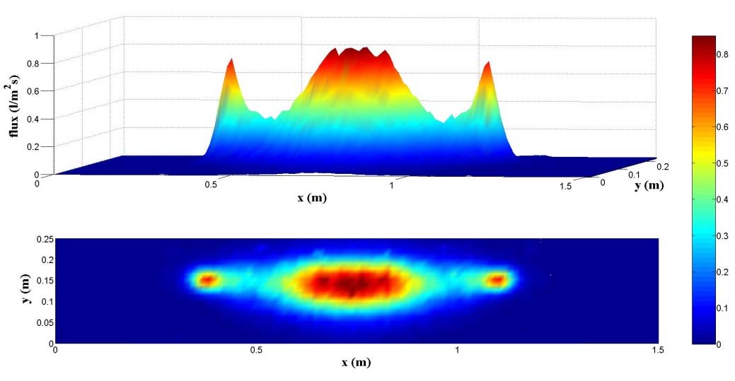
2.4 PLIF patternation
Similar to the PLIF velocimetry approach, the laser is turned 90 degrees to be orthogonal to the axial direction of the spray. Approximately 10,000 images are taken and averaged, as is
shown in Figure 10. Depending on the density of the spray, it may not be possible to
permeate the entire spray cross-section, making it necessary to assume symmetry.
Optical patternation techniques are particularly useful when the fluid to be sprayed is
hazardous. This can occur, for instance, when spraying active herbicide formulations. The
authors’ lab uses a transparent ventilated spray enclosure, constructed of acrylic and glass, to protect personnel from contact with the hazardous fluid. The sprayed liquid is fully
collected and optionally recycled in order that the amount of waste generated in an
experimental series is reduced. The enclosure is also useful for high mist-generating sprays to prevent mist accumulation onto sensitive electronic equipment.
Fig. 10. Patternation results from the averaging of 10K PLIF images.
232
Applied Computational Fluid Dynamics
2.5 Mie scattering for scalar mixing
In cases where the measurement of gas motion and scalar mixing are important to
characterize the spray, a fog has been employed to mark the gas flow. In one such method,
air is fed to the system which has first been passed sequentially through aqueous solutions
of hydrochloric acid (HCl) and ammonium hydroxide (NH3OH), which efficiently generates
a fog of ammonia droplets. This was employed in the apparatus shown in Figure 11. In this
case, the fog was introduced in a shroud around the spray nozzle. Commercial oil-
atomizing or glycerin-atomizing devices are also available to generate fogs. Smoke-
generating testing devices, used to test for negative pressure, can also be employed to
qualitatively view the air flow induced by a spray.
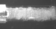
Fig. 11. Mie scattering of a shroud fog introduced around a spray nozzle to examine scalar mixing. The spray nozzle was off when this image was taken.
2.6 Mechanical patternation
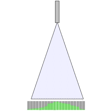
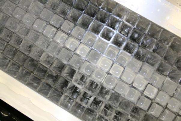
The authors have utilized both one-dimensional and two-dimensional mechanical
patternation techniques. For sprays with relatively small flowrates (< 0.5 gpm), an
arrangement of ½” x ½” cuvettes has been utilized to look at two-dimensional patterns. A
hinged door covers the cuvettes until the desired flow conditions through the spray nozzle
have been established, then the door is rapidly opened. As the fastest-filling cuvette(s)
approach full level, the door in returned to its original position and flow is stopped. The
contents of each cuvette is then carefully weighed. Figure 12 shows the method and results.
Sometimes, 2-D patternation is desired to look at subtleties in the flow pattern at the outside edges and to look at, for instance, turbulence history indicators in the sprayed solution. One such example is spraying of emulsions to study drop size distribution of an oil phase before and after spraying as a function of position in the patternator.
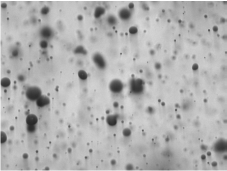
2.7 Dynamic image analysis
We have used this method to capture images of the spray droplets which are then processed
in real time. A strobe is used to backlight the imaged area, which is typically of dimensions near 1 cm x 1 cm. Out-of-focus drops are removed from the analysis by defining a sharpness
criterion for the droplet. Partial drops, extending beyond the edge of the images, are also
removed. Non-spherical droplets are converted to an equivalent diameter by matching the
projected area. A sufficient number of images are taken at 30 Hz to achieve converged drop
size distribution, commonly 50,000 to 100,000 validated drops. The frequency can be
adjusted based on expected drop velocity to assure that the same drops are not counted
more than once. Figure 13 shows a sample image taken from dynamic image analysis of a
flat fan agricultural spray.
Industrial Sprays: Experimental Characterization and Numerical Modeling
233
This type of size analysis is commonly used in the authors’ lab for nozzles with relatively small-scale flows, although the nozzle test stand of Figure 1 also uses this type of drop size analysis.
1.2
1.2
1
1
0.8
0.8
2
2
Flux, lit/s/m
0.6
Flux, lit/s/m
0.6
0.4
0.4
0.2
0.2
0
0
6
0
6
0
.3
5
5
.3
0
5
0
0
.3
.3
5
.2
0
-0
.2
5
.2
5
-0
.2
-0
-0
.1
-0
.1
5
-0
.1
.1
-0
-0
.0
00
-0
.0
00
05
5
-0
0
5
S1
-0
S1
-0
0.
10
-0
10
0.
1
5
-0
0.
1
0.
20
0.
20
0.
2
0.
25
0.
30
0.
30
0.
36
0.
36
0.
0.
0.
0.
Distance from centerline, m
0.
Distance from centerline, m
1.4
1.4
1.2
1.2
1
1
0.8
0.8
2
Flux, lit/s/m
2
Flux, lit/s/m
0.6
0.6
0.4
0.4
0.2
0.2
0
0
1
6
1
6
.4
0
0
.3
5
5
.3
0
5
0
.4
.3
0
5
-0
.2
5
.3
0
-0
.2
5
-0
.2
0
-0
.2
-0
.1
.1
-0
.1
5
-0
.0
0
-0
.1
00
-0
05
-0
.0
-0
10
S1
-0
0
S1
-0
0.
5
-0
10
5
0.
15
0
15
0.
20
-0
-0
0.
20
0.
2
0.
2
6
0.
3
0.
30
0.
36
0.
3
0.
41
0.
41
0.
0.
0.
Distance from centerline, m
0.
0.
0.
Distance from centerline, m
Fig. 12. Mechanical patternation. Upper left, general concept. Upper right, filled cells from a 2-D patternation measurement of a flat fan spray. Middle images, 2-D patternation results from a Spraying Systems Co. Teejet 8002 nozzle under identical conditions except for a
formulation change to the sprayed liquid. Bottom images, Teejet 8002E nozzle at same
conditions as the Teejet 8002 in the middle images.
234
Applied Computational Fluid Dynamics
Fig. 13. Sample dynamic image from an agricultural spray.
2.8 Summary of experimental methods
The analytical needs of the researcher varies from spray to spray and project to project. In some cases, only verification of spray angle is needed for a custom industrial installation or for a series of similar but slightly different nozzles. At the other end of the extreme, there are situations where information on velocity profile, drop size, and mass flux distribution are
needed to parameterize the inputs to a CFD model. In other cases, the impact of changes in
formulation need to be elucidated based on changes to film breakup dynamics and drop
size. The experimental tools described here have been able to provide the required
information for a wide variety of industrial problems encountered.
3. Computational methods for spray analysis
In last two decades, several attempts have been made using Eulerian-Lagrangian (E-L)
computational fluid dynamics (CFD) based models for simulating spraying. However, well
established E-L CFD models for fluid flow and evaporative/reactive spray dynamics are
sensitive to spray origin parameters, such as initial droplet size distribution, initial velocity and droplet number density. These spray origin parameters are controlled by primary
atomization. Advanced mathematical models for primary atomization are needed to
compute time-averaged and transient characteristics of droplet formation. Recent advances
have been made using computational model for developing better understanding on the
primary atomization process (Gorokhovski and Herrmann, 2008; Bini et al., 2009; Herrmann
et al. 2011). However, these studies demand significant computational time and resources
even for idealized flow conditions (e.g. nonreactive system).
3.1 Primary atomization
3.1.1 Eulerian-Eulerian approach for modeling primary atomization
In the Eulerian-Lagrangian approach for modelling spray behavior, the atomization process
is typically modelled using a surface wave instability model that predicts spray parameters
such as the spray angle and droplets’ diameters. The surface wave growth models widely
used include the surface wave instability model [Reitz and Diwakar], the Kelvin-
Helmholtz/Rayleigh-Taylor (KHRT) instability model [Patterson and Reitz] and the Taylor
Analogy Breakup (TAB) model [O’Rourke and Amsden]. The effect of nozzle geometry on
the primary atomization is approximated using an empirical nozzle-dependent constant,
Industrial Sprays: Experimental Characterization and Numerical Modeling
235
which require experimental data or experience to give reliable predictions. With the high
performance computing (HPC) system becoming more powerful and less costly in recently
years, it is becoming more feasible to directly model the primary atomization by resolving
the gas-liquid interface evolution and breakup use an Eulerian-Eulerian approach
[Gorokhovski and Herrmann].
Immiscible fluids interface tracking can be done using several approaches in the Eulerian
framework: the front tracking method [Unverdi and Tryggvason, 1992], the volume of fluid
(VOF) method [Hirt and Nichols, 1981] and the level set method [Osher and Sethian 1988,
Sussman 1994]. The front tracking method, which tracks the motion of the surface marker
particles attached to the gas-liquid interface, has numerical limitations for three-dimensional irregular interfaces. It is therefore not popularly used for predicting primary atomization. In the VOF method, the volume fraction of a fluid (i.e. the liquid phase) is solved for each of the computational cells:
V ∙
0 (1)
, , ,
(2)
The nature of the VOF model ensures mass conservation. Because the method takes a
volumetric approach to track the interface motion, numerical diffusion is inevitably inherent in the model. Special numerical algorithms are available for reconstructing the interface
shape and minimizing the numerical diffusion [Youngs 1982, Ubbink 1997, Muzaferija et. al.
1998]. Surface tension is typically implemented as a volumetric force using the continuum
surface force (CSF) method [Brackbill et. al. 1992].
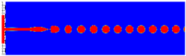
Figure 14 shows the predicted jet breakup to form droplets for a laminar jet using the VOF
method, showing good agreement with the measured droplet sizes.
In the level set method, a scalar equation representing the signed distance from the interface is solved:
V ∙
0 (3)
The interface is described with the zero level curve of the scalar. For ensuring the scalar
function to remain the signed distance to the gas-liquid interface, a redistancing algorithm is typically applied. This can generate mass loss in under-resolved regions. This can be reduce by refining the computational mesh for avoiding under-resolved regions or taking the
coupled level set VOF (CLS) approach [Mikhael Gorokhovski and Herrmann, 2008]. Figure
15 gives a snapshot of the predicted drops using the coupled level set VOF method
[Liu,Garrick and Cloeter, 2011].
Fig. 14. Predicted droplets formed due to the Rayleigh-Taylor instability using the VOF
method, showing good agreement with measured droplet sizes.
236
Applied Computational Fluid Dynamics
Fig. 15. Predicted primary atomization using the coupled Level Set - VOF method [Liu,
Garrick and Cloeter, 2011].
3.2 Coupling reaction, flow and spray dynamics
Computational implementation of coupled primary atomization, two-phase spray model,
simultaneous heat and mass transfer and subsequent reaction is a challenging and difficult
task. The major difficulty in primary atomization simulation is disparity between the time and length scales in liquid core and gas phase domain. Efficient computational approaches need to be developed to resolve the numerical stiffness due to the coupling between the jet transport equation and gas phase dynamics near nozzle. Furthermore, adequate topological
representation of the three dimensional jet core shape and the surrounding gas computational grid needs to be established. The volume of fluid (VOF) method is used to capture gas-liquid interface (Liang and Ungewitter). However, VOF requires very high grid resolution for
resolving jet surface. Therefore, including primary atomization in simulating reacting sprays become a huge challenge with respect to computational demand. In the majority of CFD
simulation of spray combustion, the atomization process is presented in terms of a point or
surface source of droplets with a prescribed size distribution introduced at the nozzle exit. The subsequent breakup and coalescence of the droplets are modelled based on the droplet Weber
number criteria. This approach uses the assumption that the dynamics and breakup of liquid
jet indistinguishable from those of a train of drops. In this work, a CFD model is presented using the above described approach to simulate reacting spray dynamics.
The particle formation in the fluid bed reactor is a complicated process involving
multiphysics. It is affected by many factors such as the dispersion of catalyst drops, the
solvent evaporation rate (if it is used for dissolving solid catalyst), the mass transfer of reactant gas into the catalyst drops and the reaction kinetics. The nozzle operating
conditions and design of the injection nozzle control the dispersion of catalyst droplets in the dilute zone. Whereas, the mass transfer to and from the droplets and the interaction
between the droplets are controlled by the quality of droplet dispersion in the dilute zone.
This indicates complex interactions between the operating conditions (shroud velocity),
Industrial Sprays: Experimental Characterization and Numerical Modeling
237
reactor hardware (nozzle design) and performance (dispersion of droplets and rates of
transport processes). Due to the complex physics involved, it is advisable to break the
complex process into multiple simpler sub-processes for better understanding of their
effects on the overall process. The above discussed problem is broke into two parts. In the
first part, CFD model was developed to understand the influence of the operating
conditions and prevailing fluid dynamics o