particularly aggressive (Oshima e al., 2001).
Therefore, the possibility of predicting cavitation is fundamental in hydraulic components
design and both experiments and numerical simulation have to be employed and integrated
in order to help the understanding of the basics of cavitation occurrence. Particularly,
numerical analysis can provide a great amount of data that can extend the experimental area
and deepen the insight of the physical phenomenon (Yang, 2002, 2005). Nevertheless, the
accuracy and reliability of the numerical models have to be addressed when approaching a
new problem or when they are modified to account for a more detailed description of the
physical process. The model sensitivity with respect to the fluid-dynamics characteristics of the case studied (such as the Reynolds number in the critical sections, the geometry
250
Applied Computational Fluid Dynamics
complexity and the boundary conditions) must be properly addressed before adopting the
numerical tool as a predictive design tool.
When addressing numerically the flow through the metering section of hydraulic
components, particular care should also be devoted to the operating conditions accounted
for in the simulations. In fact, the behaviour of the flow is usually highly time dependent, as well as the geometry of the component varies according to the working conditions. Thus,
the choice of carrying out a steady state or a fully transient CFD simulation of the
component is a critical issue in the design methodology. On one hand, the former approach
is characterized by a significantly lower computational effort as well as a shorter case setup time, but it evaluates the fluid-dynamics performance of the hydraulic component only
under the assumption of steady state operation, which is often a very limiting restriction
compared to the real operations. Conversely, the fully transient CFD calculation predicts
more accurately the real behaviour of the flow within the hydraulic component, but the
required computational effort is remarkably large and both the setup time and the
simulation execution duration can be considerably long. Therefore, it is important to
highlight the quality of the results that can be obtained by performing these two types of
CDF simulations, in order to select the correct approach for each analysis that has to be
carried out.
In this chapter, the above mentioned critical aspects in the application of multidimensional numerical analysis for the design of mechanical devices and components for hydraulic
systems are addressed. The objective of the chapter is to provide a roadmap for the
multidimensional numerical analysis of the hydraulic components to be used effectively in
the design process. In particular, two examples of hydraulic systems are accounted for in the application of the CFD analysis: a proportional control valve and a fuel accumulator for
multi-fuel injection systems. These test cases have been selected due to their
representativeness in the field of hydraulic applications and to the complexity and variety of the physical phenomena involved.
2. Prediction capabilities of the numerical models
The Navier–Stokes equations for isothermal, incompressible flows are solved by means both
of the open source multidimensional CFD code OpenFOAM (OpenCFD, 2010,
OpenFOAM®-Extend Project, 2010), and the commercial CFD code ANSYS CFX. Bounded
central differencing is used for the discretization of the momentum, second-order upwind
for subgrid kinetic energy. Pressure–velocity coupling was achieved via a SIMPLE similar
procedure. The second-order implicit method is used for time integration scheme. No time
integration scheme is involved, and all the calculations are performed under steady state
conditions.
In the modeling of the turbulent cases the performance of three turbulence models are
investigated:
1. The standard k-ε model (KE), including wall functions for the near-wall treatment;
2. the a low-Reynolds number model developed by Launder and Sharma (LS), (Launder &
Sharma, 1974) in which the transport equations for the turbulent quantities are
integrated to the walls;
3. the two zonal version of the k-ω model, known as the shear stress transport model (SST)
(Menter, 1993).
Multidimensional Design of Hydraulic Components and Systems
251
Since the objective of this investigation is the analysis of confined flows, the attention is paid to near-wall behaviour, to the damping functions and to the boundary conditions. Hence the
choice of addressing the predictive capabilities of turbulence models with a different near
wall treatment is made. In the k- model, the transport equations are not integrated to the
walls. Instead the production and dissipation of kinetic energy are specified in the near-wall cell, using the logarithmic law-of-the-wall. The validity of the near wall treatment requires that the values of the y must be in the range between 30 and 100. In the k- ε model formulation proposed by Launder and Sharma the definition of the turbulent kinetic energy
dissipation is modified to account for the low Reynolds regions close to the wall. In fact, this equation is solved for instead of ε, and a new term E is added to compensate for additional production and to further balance diffusion and dissipation in the vicinity of the walls. In this way, the Launder and Sharma approach has the advantage of the natural
boundary condition 0 at the walls. The model’s constants are the same as the standard formulation, but the damping factor functions are evaluated as a function of the turbulent
Reynolds number. The boundary conditions at the wall are k 0 and 0 . For the low Reynolds number turbulence models the requirement on the y values is more stringent, in fact y should never be larger than one. The. shear stress transport model is derived from the original two zonal version of the k-ω model proposed by Wilcox (Wilcox, 1988), and
based on the transport equation proposed by Kolmogorov. In this model the damping
functions in near-wall regions are not necessary. The eddy viscosity is calculated as the ratio between the turbulent kinetic energy and the the specific dissipation, . The original version of the model demonstrated to be very sensitive to specified in the free-stream (Menter,
1994). Therefore a new formulation was proposed by Menter combining the the k- model
by Wilcox in the inner region of the boundary layer, and the standard k - ε in the outer
region and the free-stream. The equation differs from the one of the original k- model
because of an additional cross-diffusion term. In the inner part of the boundary region the
model’s constants are the same as the k-ω model, while in the outer region they become
similar the k–ε ones. The boundary conditions do not change from the original k- model
formulation, and similarly require y smaller than 3. In this analysis careful attention was paid in order to comply with the requirements on the y values for the different turbulence models adopted.
2.1 Flow through a circular pipe
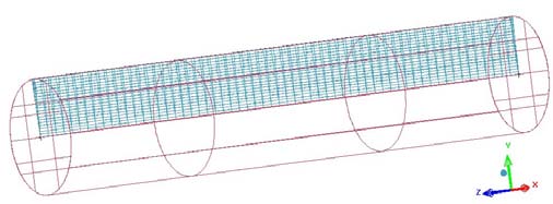
First phase of the analysis is the simulation of the fundamental test case represented by the flow through a circular pipe. The geometrical domain is assumed to be a straight circular
pipe, characterized by an axial length equal to 1.0 m and a diameter of 10 mm, pure water is considered as the operating fluid and both laminar and turbulent conditions are accounted
for. Due to the axial symmetry of both the geometry and the boundary conditions, the
simulations assume a two dimensional domain. Therefore, the meshes are defined as
circular sectors with an angular amplitude equal to 5° (see Fig.1).
A preliminary sensitivity analysis with respect to the grid resolution is carried out, in order to assess the best compromise between the accuracy of the results and the computational
cost. Different grids are constructed varying the cell spacing both in the axial and radial
direction. For the laminar case, the cell axial dimensions equal to 1.0, 2.5, and 10 mm are
compared keeping constant the resolution along the cylinder radius (i.e. 0.3 mm); whereas
the grids used in the turbulent case are characterized by a radial cell size equal to 0.3, 0.1
252
Applied Computational Fluid Dynamics
Fig. 1. 2D mesh for the straight circular pipe
Grid
Turbulence
Case #
CFD code
(ax. & rad.)
Model
A_1; A_2; A_3; A_4
FOAM
1.0x0.3; 2.5x0.3; 5.0x0.3; 10.0x0.3
Laminar
A_5; A_6; A_7; A_8
CFX
1.0x0.3; 2.5x0.3; 5.0x0.3; 10.0x0.3
Laminar
A_9; A_10; A_11
FOAM
5.0x0.05; 5.0x0.1; 5.0x0.3
LS
A_12; A_14; A_16
CFX
5.0x0.05; 5.0x0.1; 5.0x0.3
KE
A_13; A_15; A_17
CFX
5.0x0.05; 5.0x0.1; 5.0x0.3
SST
Table 1. List of simulations for the laminar and turbulent flow through the circular pipe
and 0.05 mm and a constant axial dimension (i.e. 5 mm). The meshes consist only in
hexahedrons and prisms along the cylinder axis; the height of the cells near the walls is
carefully chosen in order to comply with the requirements of the turbulence models used in
the simulations on the distance to the wall of the first node. Table 1 shows the
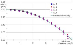
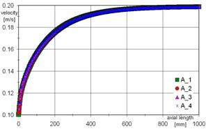
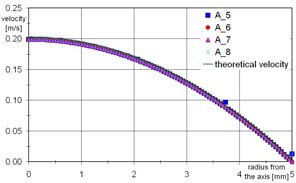
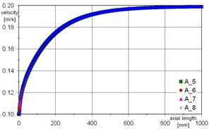
comprehensive list of the simulations performed. For the laminar cases a fluid axial velocity of 0.1 m/s is set at the inlet boundary, while a static pressure boundary condition was
considered at the pipe outlet. The numerical results for the laminar regime were compared
with the Hagen-Poiseuille theory (Pao, 1995), that is applicable when no relative motion
between the fluid and the wall appears, and an incompressible Newtonian fluid undergoes
to a isothermal laminar flow. Under these assumptions, the axial velocity profile versus the distance from the axis can be determined from the expression:
1
p
v
2 2
0
r
r
4
(1)
z
As well known, the laminar velocity assumes the fully developed profile at a distance from
the pipe inlet on the basis of the Langhaar length, defined as:
'
L 0.058 Re D
(2)
In Figs. 2 a) and c) the theoretical axial velocity profile as a function of the distance from the cylinder axis is compared with the calculated profiles for the different grid resolutions. Both codes used in the simulations demonstrated a good agreement with the axial velocity profile
derived from the Hagen-Poiseuille, and also demonstrated a negligible influence on the cell
dimension. Similar behaviour could be noticed in the velocity profile prediction, see Figs. 2
b) and d), and practically no differences could be seen among the simulated cases.
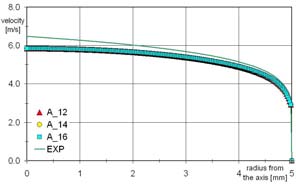
When investigating the flow field under fully turbulent conditions a fluid axial velocity of 5.0 m/s was set at the inlet boundary. Calculations were performed for three grids having
Multidimensional Design of Hydraulic Components and Systems
253
different cell dimensions, and the performance of the turbulence models described in the
previous sections (i.e. the standard k - model, the k – ω shear stress transport model and the low Reynolds Launder-Sharma models) is investigated. The results were compared
with the experimental measurements performed by Nikuradse available in literature (Pao,
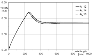
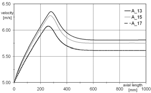
1995). In Figs. from 3 to 5 the axial velocity versus the distance from the cylinder axis and the cylinder outlet are depicted. The KE model demonstrated a good agreement with the
measurements and a scarce sensitivity to the grid size; in particular the logarithmic law-
of-the-wall was able to capture the curvature of the axial velocity in proximity to the wall.
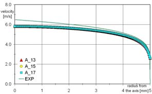
Whereas, the SST model resulted to be remarkably more influenced by the mesh
resolution. In fact Fig. 4 b) shows that the predicted axial velocity differs significantly for the three simulated grids. In particular the coarser grid calculation underestimates the
velocity magnitude, while the discrepancy between the curves relating the fine and
intermediate meshes are less evident and closer to the results found for the KE model. The
more evident sensitivity of the SST model to the grid size is due to the stricter
requirement on the distance of the first grid node to the wall. The sensitivity to the mesh
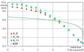
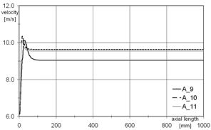
resolution was found to be even more marked for the LS model (see Fig. 5). In this model,
in fact, the transport equations are integrated up to the wall and the effect of the near wall cell is more directly transferred to the inner domain. This model demonstrated to
overestimate the axial velocity in the core region as a consequence of the velocity
magnitude tendency when approaching the wall boundary. The dissipation of the
turbulent kinetic energy is therefore overestimated and the model constant should be
tuned accordingly. For the present study the constants of the considered models were
kept the same as the suggested values.
a)
b)
c)
d)
Fig. 2. a) and c) Axial velocity profile vs. the distance from the axis and b) and d) axial
velocity profile along the cylinder axis vs. the distance from the pipe inlet: comparison
among different grid resolutions (laminar regime)
254
Applied Computational Fluid Dynamics
a)
b)
Fig. 3. a) Axial velocity profile vs. the distance from the axis and b) Axial velocity profile along the cylinder axis vs. the distance from the pipe inlet: comparison among different grid resolutions (KE model)
a)
b)
Fig. 4. a) Axial velocity profile vs. the distance from the axis and b) Axial velocity profile along the cylinder axis vs. the distance from the pipe inlet: comparison among different grid resolutions (SST model)
a)
b)
Fig. 5. a) Axial velocity profile vs. the distance from the axis and b) Axial velocity profile along the cylinder axis vs. the distance from the pipe inlet: comparison among different grid resolutions (LS model)
2.2 Flow through a small sharp-edged cylindrical orifice
Further step of the analysis is the investigation of the flow pattern through a sharp-edged
cylindrical orifice. Although the geometry of this test case is very simple, it well represents the fluid-dynamics conditions which can be found in the critical sections of many hydraulic
components. In addition, experimental measurements of the flow through abrupt section
change in circular pipes are available in literature. Therefore, it is possible to address the predictive capabilities of the numerical calculations by comparing the main flow

Multidimensional Design of Hydraulic Components and Systems
255
characteristics with experiments. In the present work the measurements carried out by
Ramamurthi and Nandakumar in 1999 were taken as a reference. In the experiments, with
reference to pure water, the effects of varying the diameters of the sharp-edge orifice and the ratio of the inlet diameter ( d) and the orifice length ( l) are investigated for different Reynolds numbers of operation. The experimental set-up consisted of a tank for the water, a nitrogen
gas source for pressurizing the tank and a feed-line fitted with flow control valves for
supplying water to the orifice. The modelling of the experimental device focuses only on the orifice geometry, and particular care is paid to assure that the flow at the orifice extremes is not influenced by the inlet and outlet of the CFD domain. To do this, two plenums are
considered at the orifice inlet and outlet, each one having a diameter and an axial length ten times larger than the orifice diameter. Thanks to the axial symmetry of the geometry and of
the boundary conditions, it is possible to account only for a 5° sector of the whole domain, and to simulate the experiments as two dimensional cases. Fig. 6 shows an example of the
CFD domain used. The simulations accounted for three orifice diameters (i.e. 0.5, 1 and 2
mm), three aspect ratios (i.e. 1, 5 and 20) and different Reynolds numbers. The complete list of the simulations, together with their main features, is detailed in Table 2.
Fig. 6. CFD domain for the small sharp-edged cylindrical orifice test case
Turbulence
Case #
Section diameter
l/d
Reynolds number
Model
B_1; B_4; B_7
0.5; 1.0; 2.0 mm
1
5x10³; 1x10⁴; 2x10⁴
KE
B_2; B_5; B_8
0.5; 1.0; 2.0 mm
5
1.1x10⁴; 2x10⁴; 4x10⁴
KE
B_3; B_6; B_9
0.5; 1.0; 2.0 mm
20
2x10⁴; 4x10⁴; 6x10⁴
KE
B_10; B_13; B_16
0.5; 1.0; 2.0 mm
1
5x10³; 1x10⁴; 2x10⁴
SST
B_11; B_14; B_17
0.5; 1.0; 2.0 mm
5
1.1x10⁴; 2x10⁴; 4x10⁴
SST
B_12; B_15; B_18
0.5; 1.0; 2.0 mm
20
2x10⁴; 4x10⁴; 6x10⁴
SST
B_19; B_22; B_25
0.5; 1.0; 2.0 mm
1
5x10³; 1x10⁴; 2x10⁴
LS
B_20; B_23; B_26
0.5; 1.0; 2.0 mm
5
1.1x10⁴; 2x10⁴; 4x10⁴
LS
B_21; B_24; B_27
0.5; 1.0; 2.0 mm
20
2x10⁴; 4x10⁴; 6x10⁴
LS
Table 2. List of simulations for the turbulent flow through a small sharp-edged cylindrical
orifice
In the modelling, the above mentioned standard k- model, the shear stress transport model
and the low Reynolds Launder-Sharma model are compared. Moreover, similarly to the
flow through a circular pipe case, different grid resolutions are tested to reduce the grid
sensitivity. Finally, a ratio between the radial cell dimension and the orifice radius of 0.02 is found to be a good compromise between computational cost and results accuracy. The
256
Applied Computational Fluid Dynamics
numerical results are compared with measurements mainly in terms of the orifice discharge
coefficients. In the experiments the discharge coefficient is calculated using the relation: 2 p
Q Cd o
A
(3)
where p
is the pressure drop across the orifice, the fluid density, A0 the orifice
geometrical area and Q the volumetric flow rate.
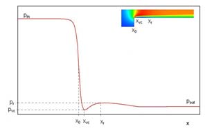
Particular care was devoted in calculating the pressure drop and, in order to assess the
influence of the abrupt section change only, it was defined as the difference between the
inlet static pressure, pin , and the static pressure at the vena contracta position, pvc .
Fig. 7. Axial pressure for the small sharp-edged cylindrical orifice test case
With reference to Fig. 7, the fluid pressure in the vena contracta section, and the axial
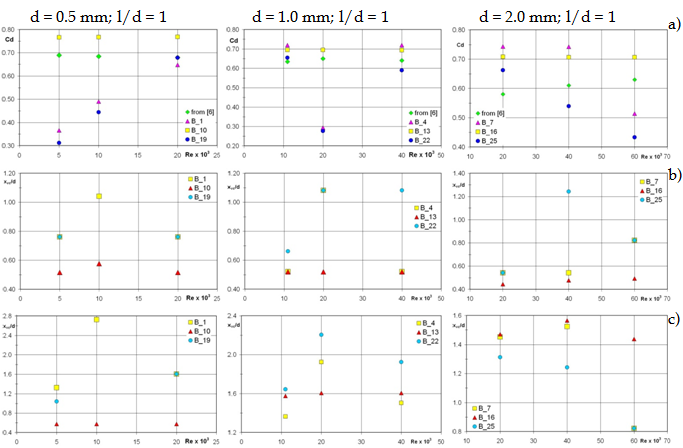
position of both the vena contracta ( xvc ) and the reattachment section ( xr ) are accurately estimated using the pressure distribution along the orifice length. In particular, the latter parameter is assumed as the axial coordinate of the relative maximum of the pressure profile downstream the vena contracta position. Fig. 8 a) collects, for all the cases reported in Table 3, the comparison between the experimental and the predicted discharge coefficients. As shown,
for a given test case and for a wide variation of the Reynolds Number, each graph directly
compares the experimental discharge coefficient with the numerical predictions obtained by
using all the turbulence models previously depicted. The agreement of the calculated
discharge coefficients and the experiments varied significantly among the test cases. The
simulations demonstrate a better predictive capability for larger aspect ratios and lower
Reynolds number. Under these conditions, the values calculated by using the KE and SST
models are sufficiently close to the measured ones. On the other hand, a worse agreement is
found for lower aspect ratios. Both turbulence models are able to capture the overall trend of the experiments, even though the SST model demonstrated a better accuracy.
While the behaviour of the KE and SST resulted to be similar, the values calculated by the
LS model are found to be significantly different from measurements, and in particular for
cases characterized by a small diameter and a low aspect ratio. The tendency of the LS
turbulence model of underestimating the velocity close to the wall (highlighted in the flow
through a circular pipe analysis also) is therefore confirmed. Consequently, the high
turbulent kinetic energy dissipation rate causes a reduced velocity in proximity to the wall, thus forcing a smaller orifice effective area. This behaviour can be noticed also when
comparing the axial coordinate of the vena contracta and of the reattaching point calculated by using the three turbulence models (see Fig. 8 b) and c) ). A similarity can be noticed for the KE and SST models: while the reattaching points calculated by the LS model result to be
Multidimensional Design of Hydraulic Components and Systems
257
Fig. 8. a) Experimental and calculated discharge coefficients and axial coordinate of b)the
vena contracta position and c) the reattaching point for different Reynolds number
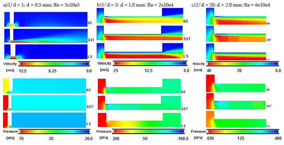
Fig. 9. Turbulence models influence on the velocity magnitude and pressure distribution
more distant from the orifice inlet. In many cases the relative maximum in the pressure
profile along the geometry axis is found to be downstream the orifice outlet. This behaviour can be explained by investigating the velocity and pressure distribution along the channel
258
Applied Computational Fluid Dynamics
(see Figs. 9). Finally, it is possible to conclude that the standard k- model and the k–ω shear stress transport models demonstrate a sufficient accuracy in calculating the discharge
coefficients for most of the analyzed cases. Contrarily, the low Reynolds Launder-Sharma
model is found to overestimate the turbulent kinetic energy dissipation, particularly in the wall proximity, thus causing an underestimation in the orifice effective area prediction. For the small diameter and low aspect ratio cases, the cavitating phenomena cannot be
neglected in order to predict with a reasonable accuracy the discharge coefficients.
3. Modelling of cavitation and aeration
Once the predictive capabilities of the numerical models for the simulation of the
incompressible flow are investigated, further step of the analysis is the modelling of the