maintain as constant as possible the pressure drop across its metering edges. This action is normally influenced by a local pressure compensator which could have either a single or a
double stage configuration, and is usually placed upstream or downstream the control valve
centre. Therefore, for a given operating position of the control valve spool, and for the flowrate across the efflux area of metering orifices the pressure drop can be maintained constant independently by the actuator work-load. Fig. 15 depicts the closed centre load-sensing
proportional control valve studied here. It is designed for operational field limits up to 100
l/min as maximum flow-rate and up to 350 bar as maximum pressure. As shown, the centre
presents a Z connection between the high pressure port (P, in red) and the internal volume
(P1, magenta), which is metered in all spool directions by a twice notched edge. At the same time, both connections between the internal volume and the actuator ports (A and B, green),
and those between the actuators ports and the discharge line ports (T, blue) are metered by
multiple notched edges. It is worth mentioning that the central volume indicated as P1
normally hosts the local pressure compensator (not included in the sketch in Fig. 15). The
Figure presents also a view of the proportional control valve spool including a zoomed view
Multidimensional Design of Hydraulic Components and Systems
263
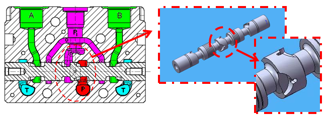
Fig. 15. Main section of the control valve and view of the spool’s metering edges
of the design of the central edge. As shown, two equal notches located at 180° characterize
each side of the central edge, and each couple of notches has a 90° rotation with respect to the other one. Moreover, the notches on the left side of the central edge meter the hydraulic power during the spool motion from the centre to the right (when P1 opens to A, and B
opens to T), while the notches on the right side works during the motion from the centre to
the left (when P1 opens to B, and A opens to T). In this way, the high pressure port P is
connected to the control valve internal volume through an asymmetric path, which depends
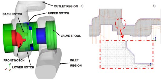
on the spool direction of motion. The CFD domain used in the simulations, see Fig. 16,
includes the metering edges of the proportional control valve (upper, lower, front and back
notch), the inlet duct and the outlet region up to the central volume where usually a local
pressure compensator is positioned. The considered domain is marked with a dashed line in
Fig. 15. The corresponding mesh is created using an unstructured grid paying particular
care to the metering areas. Local refinements are used to obtain a large number of cells in
the critical sections and at small opening positions. Moreover, wall cell layers are employed in order to have the proper wall cell height accordingly to the adopted turbulence model.
The average mesh resolution is set to 0.3 mm corresponding to an overall cell number equal
to 3 million elements. Fig. 16 b) shows the mesh of the zoomed views of a the metering edge.
In the numerical analysis, several spool positions are considered in order to simulate
different operating conditions of the control valve. In particular five spool displacements are investigated when the inlet and outlet regions are connected by means of the upper and
lower notches (i.e. direct flow through the notches) and the corresponding five spool
displacements in which the front and back notches connect the inlet and outlet of the valve
(i.e. inverse flow through the notches). The former spool positions are considered as positive while the latter ones are assumed as negative even though the opening area is the same,
since the spool displacement is symmetric with respect to the valve centre. Table 4 details all the operating conditions used in the analysis. As can be noticed from the Reynolds number
listed in Table 4, all the cases are fully turbulent. Therefore, in the simulations carried out for the present work the turbulence is modelled by means of the two zonal version of the k-ω
model, known as the shear stress transport model. Furthermore, careful attention is paid in
order to comply with the requirements of the turbulence model adopted. The results of the
numerical analysis of the load-sensing proportional control valve are discussed in terms of
discharge coefficients, pressure and velocity fields, flow forces and flow acceleration angles.
In particular the effect of the direct and inverse flow through the notches is highlighted. Fig.
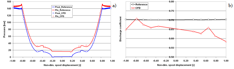
17 a) depicts the comparison between the reference and calculated inlet pressures. In the
simulations the outlet pressure is assumed as a constant boundary condition, while the inlet
264
Applied Computational Fluid Dynamics
Fig. 16. a) The geometry of the control valve included in the CFD domain and b) detail of the mesh in the notch region for a mid range opening position of the spool
Spool
displacement
Reynolds
(x/xmax)
number
-1.00 3573
Inverse flow
-0.78 4209
through the front
-0.65 3289
and back notches
-0.50 2174
-0.35 1422
0.35 1423
Direct flow
0.50 2176
through the upper
0.65 3290
and lower notches
0.78 4210
1.00 3561
Table 4. Spool displacements and operating conditions used in the simulations
pressure is calculated as a consequence of the fluid – dynamics losses through the metering
edges. As a first result, it can be noticed that even though the boundary conditions are
symmetrical with respect to the control valve centre, the predicted inlet pressure is slightly different when comparing the direct and inverse flow. This behaviour is more evident when
comparing the discharge coefficients, see Fig. 17 b). The discrepancy can be attributed to
two main reasons. First, in the direct flow (i.e. positive spool displacements) the effective area decreases progressively as the liquid flows through the notches up to the vena
contracta section close to the notch outlet; conversely, in the inverse flow, the area decreases abruptly at the notch entrance. Second, the front and back notches have very similar
geometrical boundaries both at the inlet and at the outlet, while the geometrical volumes
downstream the upper and lower notches differ significantly. In fact the liquid flowing out
from the upper notches is heading for the outlet boundary, whilst the flow out from the
lower notch finds a confined region causing further pressure losses. These reasons have
opposite effects on the discharge coefficient; in fact the first one would advantage the direct flow while the second reason would advantage the inverse flow. The numerical simulations
show that the trade-off between these two contrasting trends results in a better discharge
coefficient for the inverse flow. This behaviour is also confirmed when comparing the flow
Multidimensional Design of Hydraulic Components and Systems
265
Fig. 17. Comparison a) between reference and calculated pressures at the valve inlet and
outlet and b) between reference and calculated discharge coefficients
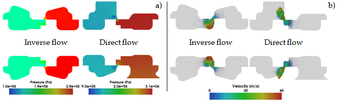
fields obtained for the different operating conditions. As an example, Fig. 18 plots the
pressure and velocity fields on a cut section through the symmetry plane of the front and
back notches (inverse flow) and the upper and lower notches (direct flow) for a small
displacement case. While the flow through the front and back notches look very similar, the
pressure and velocity fields are significantly different for the upper notch and the lower
notch. In particular, the flow exiting the lower edge hits the outlet chamber wall and
bounces back into the spool volume and then it is redirected to the outlet boundary. This
Fig. 18. a) Pressure and b) velocity distributions on a cut section through the symmetry
plane of the metering section for the inverse and direct flow (x/xmax=0.35).
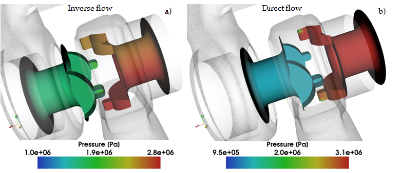
Fig. 19. Pressure distributions on the spool chambers used for the calculation of the flow
forces for a) the inverse flow and b) the direct flow)
266
Applied Computational Fluid Dynamics
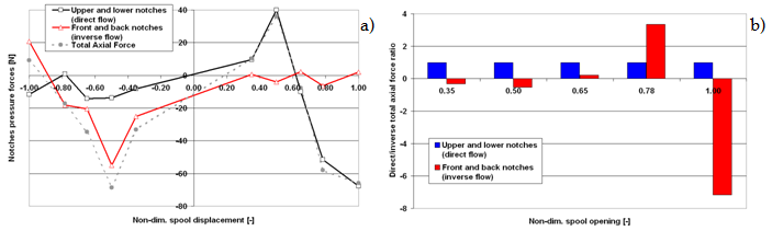
Fig. 20. a) Flow forces exerted on the valve spool in the axial direction and b) ratio between the total axial flow forces in case of direct and inverse flow
more complicated flow pattern increases the fluid – dynamics losses and thus determines a
smaller discharge coefficient. By integrating the pressure distribution over the surface of the spool chambers’ walls, it is also possible to calculate the axial forces exerted on the spool by the flow. Fig. 19 depicts the pressure contours on the walls of the spool chambers for all
notches both in case of direct and inverse flow (as an example only the case with
x/xmax=0.35 is plotted). It can be noticed that the pressure contour is quite uniform for the non operational notches, while the pressure varies significantly throughout the walls of the notches through which the oil flows. This behaviour results in a very low integrated value of the flow induced forces on the non operational chamber of the spool, as can be seen in Fig.
20. When comparing the integrated values of the forces for the direct flow (upper and lower
notches) and the inverse flow (front and back notches), it is possible to outline that the
behaviour is clearly not symmetrical with respect to the control valve centre, see Fig. 20 a).
In fact, even though the trend looks similar and in both cases the sign of the forces reverses moving from the small to the large displacements, the magnitude is rather different. Fig. 20
b) details the ratio between the total axial forces obtained in case of direct and inverse flow.
The forces have the same sign only at mid range displacements and the inverse flow
induced forces are initially lower than the direct flow ones but approaching the maximum
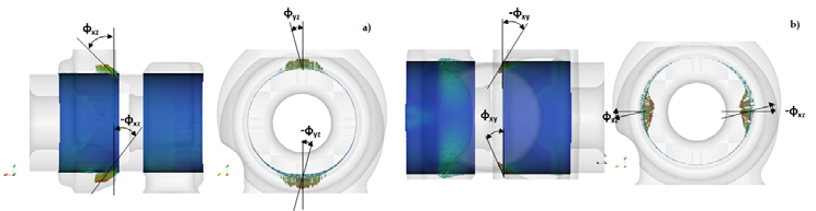
displacement they become much larger. Finally, by using the average velocity vector at the
exit of the four notches it is possible to estimate the flow acceleration angle for each
metering edge. Fig. 21 shows the convention used in this analysis for the calculation of the efflux angle with respect to the coordinate system axes. When values larger than 90 degrees
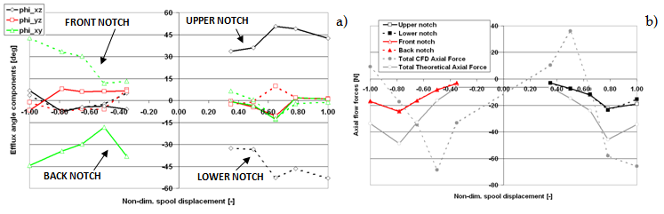
are found, the negative supplementary angle is considered. Fig. 22 a) shows the efflux
angles for the four metering sections as a function of the spool displacement. The angles are calculated for each notch only in its operational spool opening range. It is interesting to
notice that each couple of notches has a quite similar behaviour. While this result could be expected for the front and back notches due to their similar geometrical boundaries, it is less evident in the case of the direct flow, where the downstream region is very different for the upper and lower notches. Furthermore, when comparing the efflux angles obtained for the
direct and inverse flows, it can be remarked that the trend looks similar. In fact, smaller
angles are characterizing the small spool displacements, as a consequence of the Coanda
effect, whereas they are increasing moving towards the maximum opening. Nevertheless, in
the average the direct flow results in larger flow acceleration angles; this behaviour is likely due to the fact that the main flow direction change happens close to the notch exit, while in the inverse flow the stream bends abruptly just entering the notch. By knowing the flow
Multidimensional Design of Hydraulic Components and Systems
267
acceleration angles it is then possible to calculate the theoretical values of the axial forces, th
F , through the von Mises theory:
F 2
C C cos
th
d
v
p A
(7)
where Cd and Cv are the discharge coefficient and the velocity coefficient (in the following assumed equal to 0.98), Δ p is the pressure drop across the metering edge, A is its geometrical area and is the efflux angle. Fig. 22 b) depicts the comparison between the theoretical flow force and the one predicted by using the numerical simulation (grey lines). In the CFD
results, the contributions of each metering edge are also plotted (red and black lines). The theoretical calculations and the numerical predictions are significantly different, and in
particular by using the von Mises theory it is not possible to determine the change of
direction moving from low to high spool displacements both for the inverse and direct flow.
Fig. 21. Convention used for the calculation of the efflux angles
Fig. 22. a) Efflux angles for the different notches as a function of the spool displacement and b) comparison between theoretical and predicted axial forces
5. Fully transient modelling of hydraulic components
The numerical analysis of the hydraulic valve addressed in the previous section is further
deepened by adopting a fully transient numerical approach. The main issue in this type of
analysis is the moving mesh methodology employed to simulate the spool displacement
profile versus time. To accomplish this task, the mesh changer libraries of the OpenFOAM
code are modified to account for the linear motion of a portion of the geometry sliding over a second portion. The mesh motion is resolved by using a Generalized Grid Interface (GGI)
268
Applied Computational Fluid Dynamics
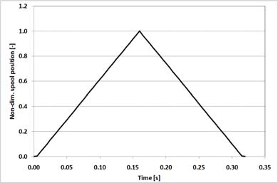
Fig. 23. PWM control applied to the spool motion
approach (Beaudoin & Jasak, 2008), originally developed for turbomachinery applications
and modified to include not only rotational motion of the moving grid but also the linear
displacement of a valve spool. The spool is moved accordingly to the PWM control profile
depicted in Fig. 23. The other models adopted in the analysis are the same as the ones
detailed in the previous sections. The valve is tested under several operating conditions. In particular, three constant flow rates at the inlet are considered, while a forth case is
accounted for, in which the pressure across the valve is held constant. The four cases are
first simulated by using a steady state approach and then a full transient approach. For the steady state simulations, four spool displacements are studied spanning from an almost
closed position to mid range and maximum displacement. In case of steady state analysis
there is no difference between the opening and the closing travels; on the contrary for the
transient approach different inertia phenomena may arise. Table 5 lists the simulated cases, detailing the steady states and transient simulations. The comparison between the results
obtained by the steady state calculations and the fully transient ones are discussed in
terms of total pressure drop across the component, discharge coefficients, pressure and
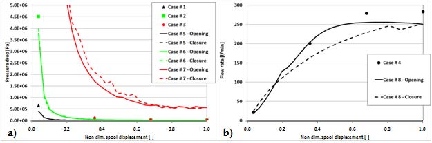
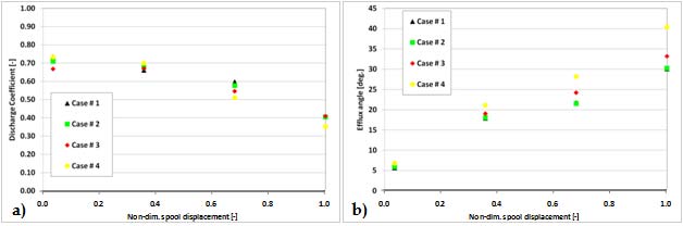
velocity fields, and flow acceleration angles. In Fig. 24 a) the total pressure drop across the valve is depicted for Cases # 1 to 3 and Cases # 5 to 7. The values predicted by the steady
state calculations and the transient ones do not differ remarkably; particularly in the
transient simulations the pressure variation during the opening and closing travels are
quite similar. A large discrepancy can be seen when considering constant pressure at the
boundaries. Fig. 24 b) plots the flow rate through the valve when holding constant the
pressure drop across the component, i.e. 20 bar. The values predicted by the steady state
simulations at small spool displacements are very close to the ones calculated during the
opening phase with the transient approach. At large spool displacement the saturation
flow rate resulted to be lower for the transient approach than for the steady state
simulation. It is interesting to notice the difference between the flow rate calculated
during the opening and the closure of the spool. The inertia of the flow through the
metering edge of the valve causes a small fluctuation as the spool reverses it direction,
while at mid range displacements the difference is even more evident. During this part of
the metering curve, the flow inertia is being opposing to the spool motion and the total
effect is a larger fluid dynamics loss. Similar behaviour can be seen also when considering
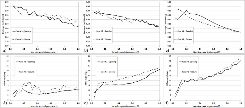
the discharge coefficients, see Figs. 25 and 26. When the flow rate is held constant, the
values during the first part of the opening travel are slightly larger than the ones during
Multidimensional Design of Hydraulic Components and Systems
269
Numerical
Inlet condition
Outlet condition
Spool positions
approach
Constant flow rate Constant pressure 0.038; 0.35; 0.68; Steady state
Case #1
(Q=12 l/min)
(pout=50 bar)
1.00
simulations
Constant flow rate Constant pressure 0.038; 0.35; 0.68; Steady state
Case #2
(Q=30 l/min)
(pout=50 bar)
1.00
simulations
Constant flow rate Constant pressure 0.038; 0.35; 0.68; Steady state
Case #3
(Q=100 l/min)
(pout=50 bar)
1.00
simulations
Constant pressure Constant pressure 0.038; 0.35; 0.68; Steady state
Case #4
(pin=70 bar)
(pout=50 bar)
1.00
simulations
Constant flow rate Constant pressure Function of time
Transient
Case #5
(Q=12 l/min)
(pout=50 bar)
(see Fig. 25)
simulation
Constant flow rate Constant pressure Function of time
Transient
Case #6
(Q=30 l/min)
(pout=50 bar)
(see Fig. 25)
simulation
Constant flow rate Constant pressure Function of time
Transient
Case #7
(Q=100 l/min)
(pout=50 bar)
(see Fig. 25)
simulation
Constant pressure Constant pressure Function of time
Transient
Case #8
(pin=70 bar)
(pout=50 bar)
(see Fig. 25)
simulation
Table 5. Boundary conditions used for the different simulated cases
closure, while as the direction reverses the discharge coefficients are larger due to the
inertia, but decreases remarkably as the metering edge reduces as an effect of the larger
losses. When comparing the discharge coefficients calculated by the steady state and
transient approach, the values are quite close, particularly at large spool displacement and for the opening travel. Conversely, if the values during the closure travel are considered, the transient simulations predict lower discharge coefficients as a results of the behaviour
mentioned before. Figs. 25 and 26 plot also the efflux angle for the different cases. The efflux angle is calculated accordingly to the reference system mentioned in section 4. A common
trend of the efflux angle is predicted for all the transient simulations. The angle tends to increase rapidly during the small spool displacements reaching a local maximum between
0.5 and 1.5 mm, ranging from small to large flow rate, while it decreases during the mid
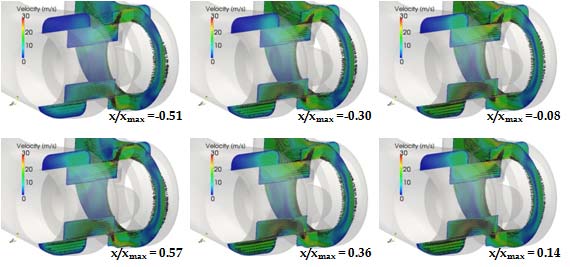
range displacements and finally it starts increasing again at high spool axial positions. The efflux angle results to be slightly larger for the closure travel all through the displacements; the flow exiting the metering section during the closure phase results to be more disperse
when compared to the flow during the opening travel. This behaviour is clearly visible
when considering the flow field during the opening and closure travels, see Fig. 27. The
efflux angle trend described above for the transient simulations is definitively different from the behaviour predicted by the steady state calculations; in fact, with the steady state
approach the efflux angle is increasing as the spool displacements increases. Furthermore,
the efflux angle values calculated by this approach resulted to be larger than the ones obtained with the transient simulations. This difference has a remarkable importance if
the flow forces are accounted for, since they are significantly affected by the vena
contracta angle.
270
Applied Computational Fluid Dynamics
Fig. 24. Comparison between the a) pressure drop and b) flow rate through the metering
area predicted by the steady state and transient simulations.
Fig. 25. a) Discharge coefficients and b) efflux angle for the steady state simulations
Fig. 26. a), b) and c) Discharge coefficient and d), e) and f) efflux angle for the transient cases
Multidimensional Design of Hydraulic Components and Systems
271
Fig. 27. Velocity distribution for different non-dim. spool displacements (Case # 7)
6. Modelling approach for a multi-fuel injection system
The numerical approach described in the previous section for the design and performance
prediction of hydraulic components is employed for the analysis of a low pressure, common
rail, multi-fuel injection system. In particular, system is working with a mean pressure close to 3.5 bar and every injector is driven by a modified PWM control characterized by 3rd
order function opening and closing ramps and characteristic times adapted to the engine
rotational speed through an ECU correction. In the numerical analysis of this hydraulic
system, the turbulence as well as the cavitation models are used to address the flow within
the injector in order to estimate the permeability characteristics of the injector when
operating with different fuels. In the analysis, the operating conditions for the injectors are preliminarily evaluated by lumped and distributed parameter approach. Thus, the system
behaviour and the injection profiles for several fuel blends are calculated. The general
reliability of the one-dimension approach is defined with respect to experimental data
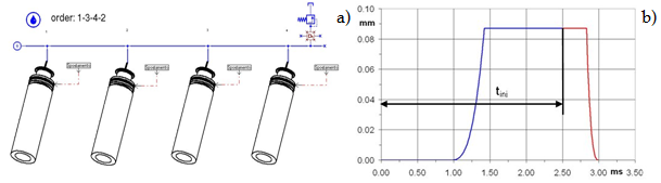
mainly in terms of injected mass per stroke. Fig. 28 shows the injection system model
including only the rail and the injectors. The connection to the supply is simplified by means of a flow-rate source. The Figure shows also the injector lift and the modified PWM wave;
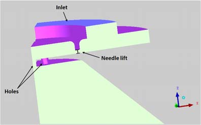
the total time, tinj, is adjusted accordingly to the measurements. The CFD analysis focuses only on the injector geometry since it represents the main component influencing the
permeability of the hydraulic system. The injector is characterized by six nozzles: the first one is in-line with the injector axis, while the other five are located circularly every 72
degrees. Therefore, the injector geometry and the boundary conditions are cyclic
symmetrical allowing the simulations to be carried out only over a 72 degree sector mesh
(see Fig. 29). In the simulations the pressure at the nozzles’ exit is kept constant equal to 1
bar, while the inlet pressure is varied from 3.5, 5 and 10 bar. In fact, the lowest inlet pressure is the current injection pressure for this type of multi – fuel injection system, but the
tendency is to increase it in order to comply with the mass flow rate required by new fuels
and new injection strategies. Finally three different fuels are accounted for in the numerical analysis. Simulations with varying needle lifts and injection pressures are carried out for
pure ethanol, pure gasoline and a fuel mixture corresponding to 50% gasoline and 50%